Simpson's Rule Integration

Introduction to Numerical Integration

Numerical Integration: A collection of algorithms employed to approximate definite integrals, particularly advantageous in scenarios where analytical integration is either complex or impractical.

• Applications in Physics:
  • Estimating the area under velocity-time graphs to calculate distance.
• Relevance in Engineering:
  • Essential in design and analysis of complex shapes and functions.

Importance of Numerical Integration

• Scenarios for Application:
  • Complex Boundary Conditions: Common in structural engineering where direct integration may not be feasible.
  • Empirical Data Analysis: For instance, using numerical methods to accurately forecast energy consumption.

Example: Numerical integration allows for the mathematical modelling of empirical data, which is beneficial for planning resources in the energy sector.

Functions Suited for Numerical Methods

• Suitable Functions:
  • Discontinuous Functions: Effectively handled using graphical methods to enhance comprehension.
  • Rapidly Changing Slopes: Such functions are accurately integrated using specific numerical techniques designed for these variations.
• Function Smoothness: Is a critical factor in selecting the most appropriate numerical techniques.

Visualising Area Approximation

• Geometric Representation:

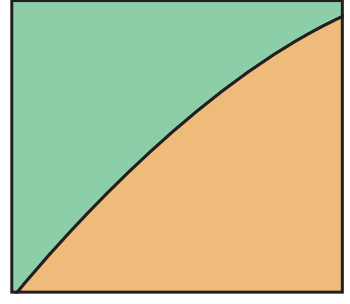  Rectangles and trapezoids provide basic approximations.

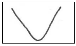  Simpson's Rule uses parabolic sections for enhanced accuracy.

• Worked Example:

  • An acceleration curve, $a(t) = t^2$, can be integrated over time using Simpson's Rule to practically demonstrate changes in velocity.

Simpson's Rule: Formula and Derivation

Simpson's Rule Formula

Simpson's Rule: A numerical technique for approximating definite integrals essential when exact solutions are unattainable, and precision in real-world applications is vital.

Basic Formula:

$S = \frac{h}{3} [f(x_0) + 4f(x_1) + f(x_2)]$

Composite Formula:

$S = \frac{h}{3} \left[ f(x_0) + 4\sum_{i=1,3,5\ldots}^{n-1}f(x_i) + 2\sum_{i=2,4,6\ldots}^{n-2}f(x_i) + f(x_n) \right]$

• h: Step size, defined as $(x_2-x_0)/2$
• x_0, x_2: Endpoint values of the interval.
• f(x_0), f(x_1), f(x_2): Function values at the respective nodal points.

Example Calculation:

• Consider $x_0 = 0$, $x_1 = 1$, and $x_2 = 2$ with $h=1$ for $f(x) = x^2$. Then: $$S = \frac{1}{3}[0^2 + 4(1)^2 + 2^2] = \frac{1}{3}[0 + 4 + 4] = \frac{8}{3}$$

Derivation of Simpson's Rule

To derive Simpson's Rule, approximate a given interval by a quadratic polynomial $ax^2 + bx + c$:

1. For the interval $[x_0, x_2]$, the function is modelled as a parabola.
2. Evaluate $\int_{x_0}^{x_2} (ax^2 + bx + c) \, dx$.
3. Integrate separately: $\int ax^2 \, dx$, $\int bx \, dx$, and $\int c \, dx$.
4. Replace terms with function values $f(x_0)$, $f(x_1)$, $f(x_2)$.

• Visual Diagram:

Examples Using Simpson's Rule

Step-by-step Example with Polynomial Function

Consider the polynomial function $f(x) = x^2 + 3x + 2$.

• Interval Selection: Divide the interval into three equal parts for simplification.
• Calculation Step-by-step:
  1. Calculate $f(x)$ at each point:
     • $f(0) = 0^2 + 3 \times 0 + 2 = 2$
     • $f(1) = 1^2 + 3 \times 1 + 2 = 6$
     • $f(2) = 2^2 + 3 \times 2 + 2 = 12$
  2. Apply Simpson's Rule:
  $$\int_{0}^{2} (x^2 + 3x + 2) \, dx \approx \frac{2-0}{6}[f(0) + 4f(1) + f(2)] = \frac{2}{6}[2 + 4(6) + 12] = \frac{2}{6}[2 + 24 + 12] = \frac{2}{6}[38] = \frac{76}{6} \approx 12.67$$
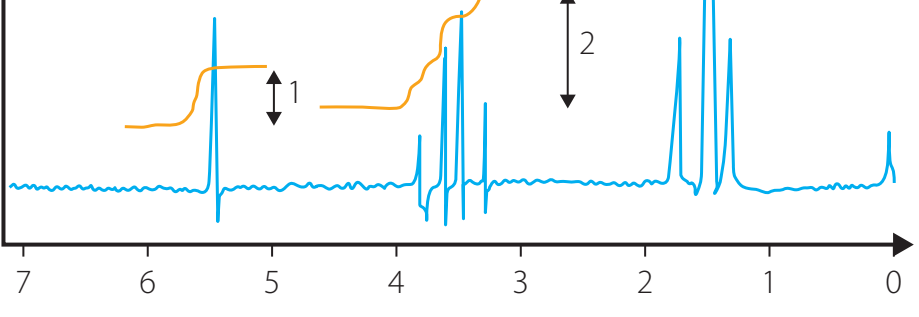
• Graphical Representation:

Example with Trigonometric Function

Applying Simpson's Rule to $f(x) = \sin(x)$:

• Interval Impact: The periodic nature of a sine wave requires careful interval selection for optimal accuracy.
• Detailed Calculation Steps:

  1. Compute over the interval $[0, \pi]$, selecting segments like 0, $\frac{\pi}{2}$, and $\pi$.

  2. Evaluate the sine function at these points and apply Simpson's Rule.

     $f(0) = \sin(0) = 0$ $f(\frac{\pi}{2}) = \sin(\frac{\pi}{2}) = 1$ $f(\pi) = \sin(\pi) = 0$

     $\int_{0}^{\pi} \sin(x) \, dx \approx \frac{\pi-0}{6}[f(0) + 4f(\frac{\pi}{2}) + f(\pi)] = \frac{\pi}{6}[0 + 4(1) + 0] = \frac{4\pi}{6} = \frac{2\pi}{3} \approx 2.094$

Graphical Aid: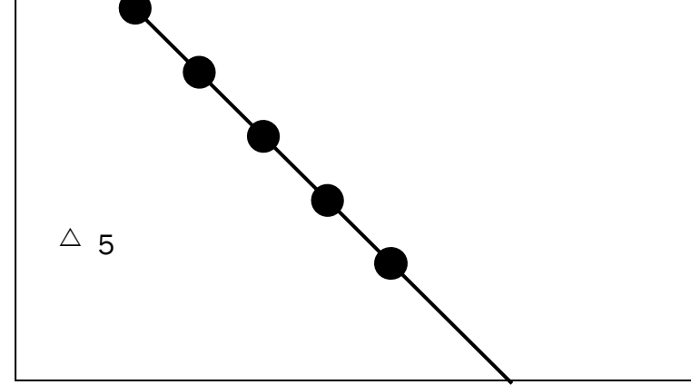

Example with Exponential Function

Consider $f(x) = e^x$:

• Calculation Steps:
  1. On the interval $[0, 1]$, select points 0, 0.5, and 1.
  2. Compute $e^0 = 1$, $e^{0.5} \approx 1.649$, and $e^1 \approx 2.718$.
  3. Apply Simpson's Rule: $\int_{0}^{1} e^x \, dx \approx \frac{1-0}{6}[f(0) + 4f(0.5) + f(1)] = \frac{1}{6}[1 + 4(1.649) + 2.718] = \frac{1}{6}[1 + 6.596 + 2.718] = \frac{10.314}{6} \approx 1.719$

Graphical Breakdown:

Simpson's Rule: Error Analysis

• Error Term:
  • Formula:
    • $E = -\frac{(b-a)^5}{180n^4}f^{(4)}(\xi)$
  • Dependency on Fourth Derivative: Indicates how the curve's nature affects accuracy.
  • Analogy: Like a road curvature affecting driving difficulty, the fourth derivative measures function 'bend.'

• Factors Affecting Error:

  • Step Size and Subintervals:
    • Smaller steps imply lower errors.
    • Doubling $n$ changes error by approximately a factor of 16.
  • Function Behaviour:
    • Smoother curves generally lead to smaller errors.

  

Comparison with Other Numerical Methods

Overview of Methods

• Simpson's Rule:

  • Pros: High accuracy due to quadratic approximations, particularly effective with smooth functions.
  • Cons: Requires an even number of intervals.

• Trapezoidal Rule:

  • Pros: Simple and practical for moderate-precision tasks.
  • Cons: Less precise than Simpson's Rule.

• Rectangular Rule:

  • Pros: Very straightforward and quick.
  • Cons: Lower accuracy for functions changing rapidly.

• Comparative Calculations:

  • Evaluate methods using polynomial: $f(x) = x^2$, trigonometric: $f(x) = \sin(x)$, and exponential: $f(x) = e^x$ to observe comparative performance.

  

Key Strategies and Tips

• Understanding Key Assumptions:

  • Continuity: Ensure the function is continuous for accurate application of Simpson's Rule.
  • Even Segmentation: Maintain even intervals.

• Common Pitfalls:

  • Errors in proper interval segmentation.
  • Misapplication of formulae and arithmetic mistakes.

• Time Management Techniques:

  • Allocate sufficient time for setup and verification of integrals.

• Worked Example:

  Problem: Use Simpson's Rule to approximate the integral of $f(x)=x^2$ from $0$ to $4$ with $n=2$ subintervals.

  • Step 1: Divide $[0, 4]$ into segments, giving points at $x_0=0$, $x_1=2$, and $x_2=4$.
  • Step 2: Calculate function values: $f(0)=0$, $f(2)=4$, and $f(4)=16$.
  • Step 3: Apply Simpson's Rule:
  $$\int_0^4 x^2 \, dx \approx \frac{4-0}{6} \left[f(0) + 4f(2) + f(4) \right]$$ $$\frac{4}{6} [0 + 4(4) + 16]$$ $$\frac{4}{6} [0 + 16 + 16]$$ $$$$

• Practice Exercise:
  • Approximate $\int_0^3 x^3 \, dx$ using Simpson's Rule with 3 subintervals.
  • Solution:
    • Step 1: Divide the interval $[0,3]$ into three equal parts giving $x_0=0$, $x_1=1$, $x_2=2$, and $x_3=3$.
    • Step 2: Calculate function values: $f(0)=0$, $f(1)=1$, $f(2)=8$, and $f(3)=27$.
    • Step 3: Apply composite Simpson's Rule:
    $$\int_0^3 x^3 \, dx \approx \frac{3-0}{3(3)} [f(0) + 4f(1) + 2f(2) + f(3)]$$ $= \frac{3}{9} [0 + 4(1) + 2(8) + 27]$ $= \frac{3}{9} [0 + 4 + 16 + 27]$ $= \frac{3}{9} [47] = \frac{141}{9} = 15.67$
    • Exact value is $\int_0^3 x^3 \, dx = \frac{3^4}{4} = \frac{81}{4} = 20.25$, so our approximation is reasonably close.

By mastering Simpson's Rule and understanding its advantages compared to other methods, students will be well-equipped to tackle numerical integration problems in their examinations.