Photo AI
Last Updated Sep 24, 2025
Second Derivative and Turning Points Simplified Revision Notes for SSCE HSC Mathematics Advanced
Revision notes with simplified explanations to understand Second Derivative and Turning Points quickly and effectively.
327+ students studying
Second Derivative and Turning Points
Defining the Second Derivative
- Second Derivative: The second derivative, represented by or , is the derivative of the first derivative.
- It describes the rate at which the slope of the graph changes, analogous to the concept of acceleration in physics.
Key Concept: The second derivative offers insight into acceleration in functions, showing how the rate of change itself varies.
Significance in Graph Curvature and Concavity
- Curvature Analysis:
- Concave Up: If , the graph "smiles," indicating positive curvature.
- Concave Down: If , the graph "frowns," indicating negative curvature.
- Example with Quadratic Function: Consider the function :
- The second derivative is positive (), showing the graph consistently smiles or remains concave up.

Introduction to Stationary Points
Importance: Stationary points are essential for analysing functions to identify changes in direction or constant regions. They are crucial in areas like physics, engineering, and economics, where they signify optimal points, such as peak demand or lowest energy states.
- Local Maximum: A point at which the function shifts from increasing to decreasing.
- Local Minimum: A point at which the function shifts from decreasing to increasing.
- Point of Inflection: A point where the curve changes concavity without reaching a true extremum.
Second Derivative Test
- Purpose and Process: The second derivative test aids in determining if stationary points are maxima, minima, or require further investigation when .
- Test Breakdown:
- If : The point is a local minimum (concave up).
- If : The point is a local maximum (concave down).
- If : Additional analysis is required.
- Begin by setting to locate potential stationary points.
- Proceed with a Second Derivative Test for classification.
Common Student Errors
- Typical Mistakes: Students may incorrectly apply the test or omit further investigation when .
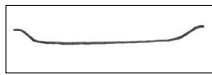
Visual Explanation: Diagrams are crucial for comprehending second derivatives and concavity.
Points of Inflection
Definition and Significance
- Point of Inflection: Point on a graph where the curve changes concavity.
- Mathematical Context:
- Signalled when the second derivative changes sign, transitioning from positive to negative or vice versa.
Example 1: Polynomial Function
Consider .
- Calculate .
- At , verify a sign change occurs.
- is an inflection point due to the sign change.
Worked Examples
Example 1: Polynomial Function
For :
- Compute .
- Set to find or .
- Calculate .
- At : (negative), so this is a local maximum.
- At : (positive), so this is a local minimum.
Example 2: Trigonometric Function
For :
- Calculate .
- Solve at ().
- Calculate .
- When : (negative), so this is a local maximum.
- When : (positive), so this is a local minimum.
Graph Sketching Using the Second Derivative
Step-by-Step Guide to Graph Sketching
1. Identify Stationary Points
- Stationary Points: Occur where .
2. Determine Concavity
- Concave Up: .
- Concave Down: .
- Assess the behaviour as approaches infinity () or negative infinity ().
Practical Application Exercises
-
Problem 1: Classify the stationary points of .
Solution:
- Find
- Set :
- Factor:
- Stationary points occur at , , and
- Calculate
- At : (negative), so this is a local maximum
- At : (positive), so this is a local minimum
- At : (positive), so this is a local minimum
-
Problem 2: Evaluate stationary points for within .
Solution:
- Find
- Since for all values in the domain, is never zero
- Therefore, has no stationary points within
- Note that has vertical asymptotes at and within this interval
Always assess endpoints and infinity behaviour for comprehensive graph sketching.


500K+ Students Use These Powerful Tools to Master Second Derivative and Turning Points For their SSCE Exams.
Enhance your understanding with flashcards, quizzes, and exams—designed to help you grasp key concepts, reinforce learning, and master any topic with confidence!
50 flashcards
Flashcards on Second Derivative and Turning Points
Revise key concepts with interactive flashcards.
Try Mathematics Advanced Flashcards5 quizzes
Quizzes on Second Derivative and Turning Points
Test your knowledge with fun and engaging quizzes.
Try Mathematics Advanced Quizzes29 questions
Exam questions on Second Derivative and Turning Points
Boost your confidence with real exam questions.
Try Mathematics Advanced Questions27 exams created
Exam Builder on Second Derivative and Turning Points
Create custom exams across topics for better practice!
Try Mathematics Advanced exam builder5 papers
Past Papers on Second Derivative and Turning Points
Practice past papers to reinforce exam experience.
Try Mathematics Advanced Past PapersOther Revision Notes related to Second Derivative and Turning Points you should explore
Discover More Revision Notes Related to Second Derivative and Turning Points to Deepen Your Understanding and Improve Your Mastery
Load more notes