Photo AI
A survey of 100 households gave the following results for weekly income $y$ - Edexcel - A-Level Maths Statistics - Question 5 - 2013 - Paper 1
Question 5
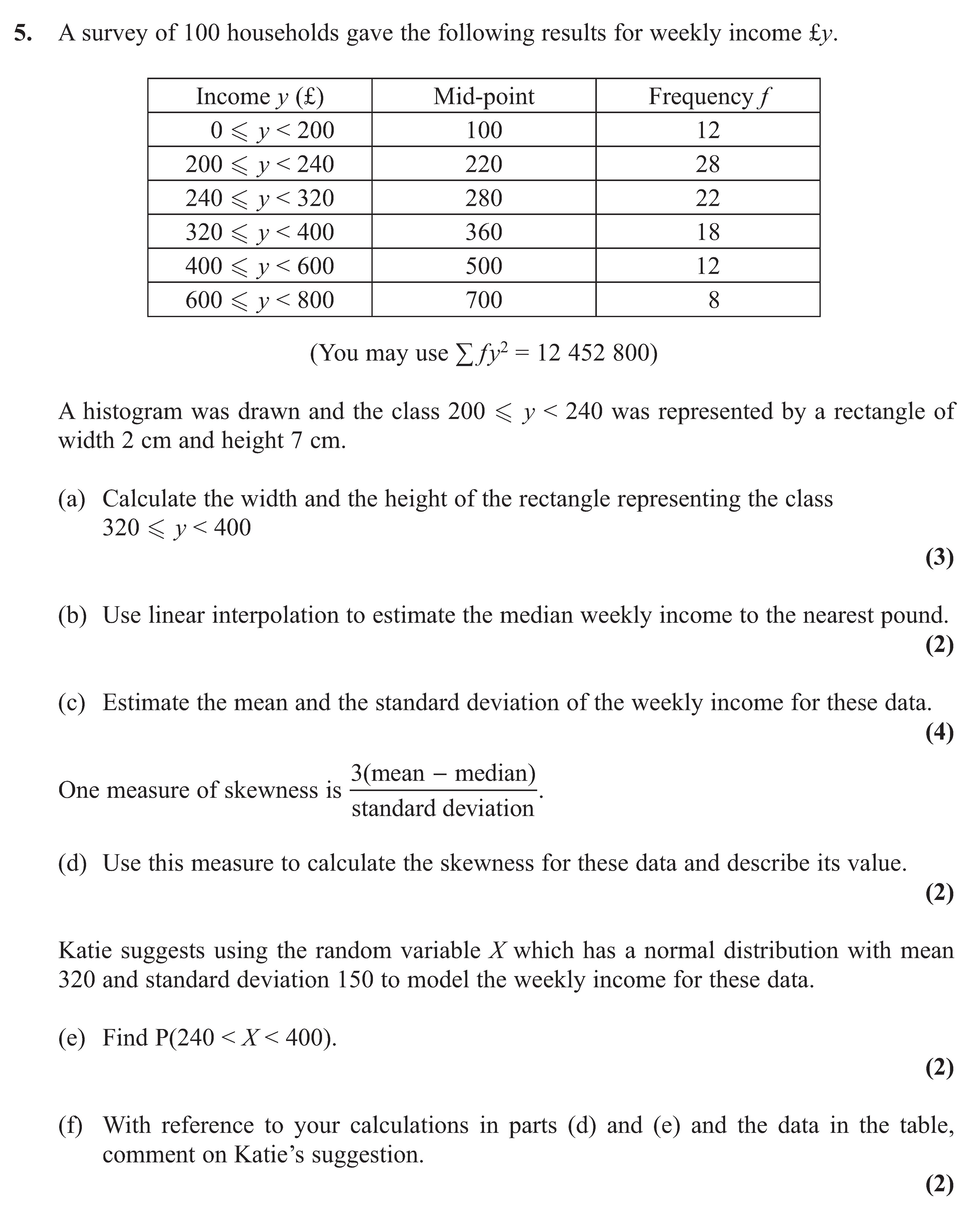
A survey of 100 households gave the following results for weekly income $y$. Income $y$ (£) $0 \leq y < 200$ $200 \leq y < 240$ $240 \leq y < 320$ $320 \l... show full transcript
Worked Solution & Example Answer:A survey of 100 households gave the following results for weekly income $y$ - Edexcel - A-Level Maths Statistics - Question 5 - 2013 - Paper 1
Step 1
Calculate the width and the height of the rectangle representing the class $320 \leq y < 400$

Answer
To find the width of the rectangle, we note that the interval from 320 to 400 is:
Width = 400 - 320 = 80
To find the height, we first calculate the frequency for the class. According to the data, the frequency for this class is 18. The area represented by a rectangle is width multiplied by height. Given that the width is 2 cm and the area represented is the frequency times the height, we set up the following equation:
Area = Frequency × Height \rightarrow 2 \times h = 18
Solving for height gives:
h = \frac{18}{2} = 9.
Therefore, the width is 80 and the height is 9.
Step 2
Use linear interpolation to estimate the median weekly income to the nearest pound.
Answer
To estimate the median, we first need to find the cumulative frequencies. The total number of households is 100, so the median corresponds to the 50th household.
Cumulative frequency:
- For class : 12
- For class : 12 + 22 = 34
- For class : 34 + 20 = 54
Since the 50th value falls in the class , we use linear interpolation:
Let , , and .
Using the formula for median:
[ Median = L + \left(\frac{\frac{N}{2} - cf}{f}\right) \cdot h ]
Substituting values gives:
[ Median = 240 + \left(\frac{50 - 34}{20}\right) \cdot 80 = 240 + 64 = 304 ]
Thus, the estimated median weekly income is approximately £304.
Step 3
Estimate the mean and the standard deviation of the weekly income for these data.
Answer
To estimate the mean, we calculate ( \sum f y = 31600 ). The mean can be calculated using the formula:
[ \text{Mean} = \frac{\sum f y}{N} = \frac{31600}{100} = 316 ]
Next, we compute the standard deviation. The formula for standard deviation is:
[ \sigma = \sqrt{\frac{\sum f y^2}{N} - \left(\frac{\sum f y}{N}\right)^2} = \sqrt{\frac{12452800}{100} - 316^2} = \sqrt{124528 - 99856} \approx 157 ]
Thus, the estimated mean is £316, and the standard deviation is approximately £157.
Step 4
Use this measure to calculate the skewness for these data and describe its value.
Answer
To calculate the skewness, we use the formula:
[ \text{Skewness} = \frac{3(\text{Mean} - \text{Median})}{\text{Standard Deviation}} ]
Substituting the known values:
[ \text{Skewness} = \frac{3(316 - 304)}{157} = \frac{36}{157} \approx 0.229 ]
This indicates a positive skew, suggesting that there are outliers on the higher income end.
Step 5
Find $P(240 < X < 400)$
Answer
In order to find the probability, we standardize the values using the Z-score formula:
[ Z = \frac{X - \mu}{\sigma} ]
Substituting for 240 and 400 gets us:
[ Z_{240} = \frac{240 - 320}{150} = -\frac{80}{150} \approx -0.533 ]
[ Z_{400} = \frac{400 - 320}{150} = \frac{80}{150} \approx 0.533 ]
Now we can find the probability using Z-table values:
P(240 < X < 400) = P(Z < 0.533) - P(Z < -0.533) \approx 0.703
- 0.297 = 0.406.
Thus, the probability is approximately 0.406.
Step 6
With reference to your calculations in parts (d) and (e) and the data in the table, comment on Katie's suggestion.
Answer
Katie's suggestion to model weekly incomes using a normal distribution based on a mean of 320 and standard deviation of 150 requires attention to the skewness calculated in part (d), which indicated a positive skew of approximately 0.229. This suggests that the income distribution is not perfectly normal, as the presence of higher incomes (outliers) skews the data to the right.
Additionally, the probability found in part (e), approximately 0.406 for incomes between 240 and 400, further emphasizes that while a normal approximation may fit broadly, the skewness and presence of outliers may render it less effective in capturing the true characteristics of the income distribution. Thus, a normal model might be approximately reasonable, yet it may not be fully adequate due to the skewness observed.