Photo AI
Last Updated Sep 26, 2025
Elasticity Simplified Revision Notes for A-Level OCR Economics
Revision notes with simplified explanations to understand Elasticity quickly and effectively.
245+ students studying
2.6 Elasticity
DEFINITION:
- Elasticity: measuring the responsiveness of demand or supply to changes in price, income or other factors
- Price elasticity of demand: the responsiveness of the quantity demanded to a change in the price of the product
- total revenue: amount of money that firms receive from selling their products
- Income elasticity of demand: the responsiveness of the quantity demanded to a change in income
- Cross elasticity of demand: the responsiveness of demand for one product in relation to a change in the price of another product
- Perfect complements: when 2 goods cannot be consumed without the other. These goods are the strongest complements because only the consumption of both goods together will provide consumer satisfaction.
- Price elasticity of supply: the responsiveness of quantity supplied to a change in price.
Explain:
2.6.1 Elasticity
Elasticity in economics measures how responsive the quantity demanded or supplied of a good is to changes in its price or other factors. Here are the key types of elasticity:
- Price Elasticity of Demand (PED): This measures how much the quantity demanded of a good responds to a change in its price. It's calculated as the percentage change in quantity demanded divided by the percentage change in price. If PED > 1, demand is elastic (consumers are very responsive to price changes). If PED < 1, demand is inelastic (consumers are less responsive to price changes). If PED = 1, demand is unit elastic.
- Price Elasticity of Supply (PES): This measures how much the quantity supplied of a good responds to a change in its price. It's calculated as the percentage change in quantity supplied divided by the percentage change in price. If PES > 1, supply is elastic (producers can increase output easily). If PES < 1, supply is inelastic (producers find it hard to increase output).
- Income Elasticity of Demand (YED): This measures how the quantity demanded of a good changes in response to changes in consumer income. It's calculated as the percentage change in quantity demanded divided by the percentage change in income. If YED > 1, the good is a luxury (demand increases more than proportionally with income). If YED < 1 but > 0, the good is a necessity (demand increases less proportionally with income). If YED < 0, the good is an inferior good (demand decreases as income rises).
- Cross Elasticity of Demand (XED): This measures how the quantity demanded of one good changes in response to a change in the price of another good. It's calculated as the percentage change in quantity demanded of Good A divided by the percentage change in price of Good B. If XED > 0, the goods are substitutes (demand for one increases as the price of the other increases). If XED < 0, the goods are complements (demand for one decreases as the price of the other increases). Understanding elasticity helps businesses and governments make informed decisions regarding pricing, production, and taxation.
Explain and calculate:
2.6.2 Price elasticity of demand (PED)
Formula:
The formula for calculating PED is:
Calculation Steps:
- Calculate the Percentage Change in Quantity Demanded:
- Calculate the Percentage Change in Price:
- Insert these values into the PED formula to determine the elasticity. Interpretation of PED Values:
- PED > 1: Demand is elastic. Consumers are highly responsive to price changes.
- PED < 1: Demand is inelastic. Consumers are less responsive to price changes.
- PED = 1: Demand is unit elastic. The percentage change in quantity demanded is equal to the percentage change in price.
- PED = 0: Demand is perfectly inelastic. Quantity demanded does not change with price changes.
- PED = ∞: Demand is perfectly elastic. Consumers will only buy at one price and none at any other price.
Example Calculation:
Suppose the price of a product decreases from 8, and as a result, the quantity demanded increases from 50 units to 70 units.
- Percentage Change in Quantity Demanded:
- Percentage Change in Price:
- Calculate PED:
Since we typically consider the absolute value, PED = 2, indicating that demand is elastic. Consumers are highly responsive to the price change.
Summary:
PED is a crucial concept in economics that helps understand how price changes impact consumer demand. It is calculated using the percentage changes in quantity demanded and price, providing insights into market behaviour and informing business and policy decisions.
2.6.3 Explanation of Income Elasticity of Demand (YED):
Income elasticity of demand (YED) measures the responsiveness of the quantity demanded of a good to a change in consumers' income. It is an important concept in economics as it helps to understand how changes in income levels affect the demand for different types of goods.
Formula:
Types of Goods Based on YED:
- Normal Goods: These are goods for which demand increases as income increases. YED is positive.
- Luxury Goods: A subtype of normal goods with YED > 1, indicating that demand is highly responsive to income changes.
- Necessities: A subtype of normal goods with 0 < YED < 1, indicating that demand is less responsive to income changes.
- Inferior Goods: These are goods for which demand decreases as income increases. YED is negative.
Calculation Example:
Suppose the income of consumers increases by 10%, and as a result, the quantity demanded for a particular good increases by 15%.
Using the formula:
Interpretation:
- YED = 1.5: This positive YED indicates that the good is a normal good and, specifically, a luxury good because the YED is greater than 1. This means that for every 1% increase in income, the quantity demanded for this good increases by 1.5%. Understanding YED helps businesses and policymakers predict how changes in economic conditions (like a rise or fall in income) will affect the demand for various goods and services.
2.6.4 Cross Elasticity of Demand (XED):
Cross Elasticity of Demand (XED) measures the responsiveness of the quantity demanded for one good when the price of another good changes. It is particularly useful for understanding the relationship between complementary and substitute goods.
Formula:
Interpretation:
- Positive XED: Indicates that the goods are substitutes. An increase in the price of Good B leads to an increase in the quantity demanded of Good A.
- Negative XED: Indicates that the goods are complements. An increase in the price of Good B leads to a decrease in the quantity demanded of Good A.
- Zero XED: Indicates that the goods are unrelated. A change in the price of Good B has no effect on the quantity demanded of Good A. Calculation Example:
Suppose the price of Good B increases from 12, and as a result, the quantity demanded of Good A increases from 50 units to 60 units.
- Calculate the percentage change in quantity demanded of Good A:
- Calculate the percentage change in price of Good B:
- Calculate XED:
Interpretation of Result:
An XED of 1 indicates that Good A and Good B are substitutes, and the quantity demanded of Good A is highly responsive to changes in the price of Good B.
Summary:
XED provides valuable insights into the relationship between different goods. A positive XED suggests substitutability, a negative XED suggests complementarity, and a zero XED suggests no relationship between the goods.
2.6.5 Price Elasticity of Supply (PES)
Formula:
Calculation Steps:
- Calculate the percentage change in quantity supplied:
- Calculate the percentage change in price:
- Calculate PES:
Example Calculation:
Suppose the price of a good increases from £20 to £25, and the quantity supplied increases from 100 units to 120 units.
- Percentage change in quantity supplied:
- Percentage change in price:
- Calculate PES:
Interpretation:
- PES > 1: Supply is elastic (quantity supplied changes more than the price change).
- PES < 1: Supply is inelastic (quantity supplied changes less than the price change).
- PES = 1: Supply is unit elastic (quantity supplied changes exactly as the price change). In this example, a PES of 0.8 means that the supply is inelastic. This indicates that the quantity supplied is relatively unresponsive to price changes. A 25% increase in price leads to only a 20% increase in quantity supplied.
Diagram:
To visualize the concept, consider the following diagram:
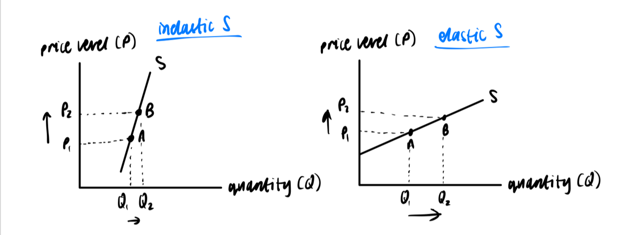
In this diagram, the upward-sloping supply curve (S) demonstrates that as the price increases, the quantity supplied also increases. However, because the supply is inelastic (PES < 1), the increase in quantity supplied is proportionally smaller than the increase in price.
Key Points:
- Elastic Supply: When PES > 1, suppliers can increase production easily with price changes, often due to readily available resources or flexibility in production processes.
- Inelastic Supply: When PES < 1, it's harder for suppliers to increase production quickly, often due to limited resources or inflexible production capacity.
- Unit Elastic Supply: When PES = 1, the percentage change in quantity supplied is equal to the percentage change in price.
Is PES likely to be positive or negative? Why?
POSITIVE → Supply curve (S) slopes upward
- More profitable to sell at higher prices
- Shows willingness and ability to sell at higher prices | PES Value | Explanation | |---|---| | Inelastic Supply | | | Elastic Supply | |
Understanding PES helps in predicting how changes in market conditions will affect supply and can guide businesses and policymakers in their decisions.
Explain with Aid of a Diagram
2.6.6 Price Elasticity of Demand (PED), Income Elasticity of Demand (YED), Cross Elasticity of Demand (XED), and Price Elasticity of Supply (PES)
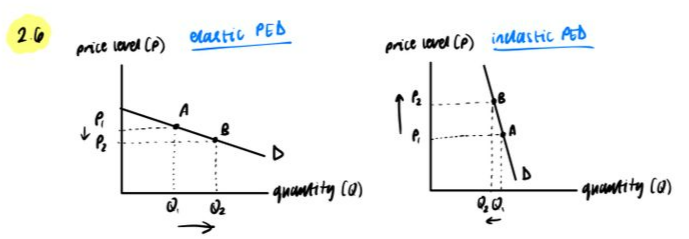
1. Price Elasticity of Demand (PED):
Definition:
PED measures the responsiveness of the quantity demanded of a good to a change in its price.
Values and Interpretation:
- PED > 1: Demand is elastic (quantity demanded changes more than the price change).
- PED < 1: Demand is inelastic (quantity demanded changes less than the price change).
- PED = 1: Demand is unit elastic (quantity demanded changes exactly as the price change).
- PED = 0: Demand is perfectly inelastic (quantity demanded does not change with price).
- PED = ∞: Demand is perfectly elastic (any change in price leads to an infinite change in quantity demanded). Diagram:
2. Income Elasticity of Demand (YED):
Values and Interpretation:
- YED > 1: Demand is income elastic (luxury goods).
- 0 < YED < 1: Demand is income inelastic (necessities).
- YED = 0: Demand is unaffected by income changes.
- YED < 0: Inferior goods (demand decreases as income increases).
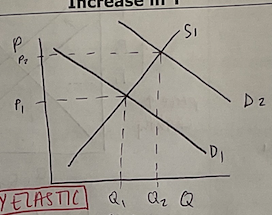
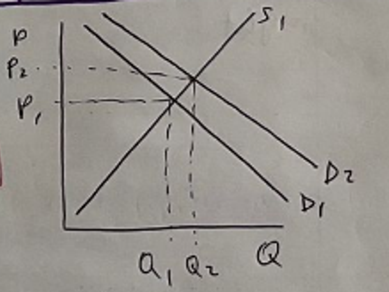
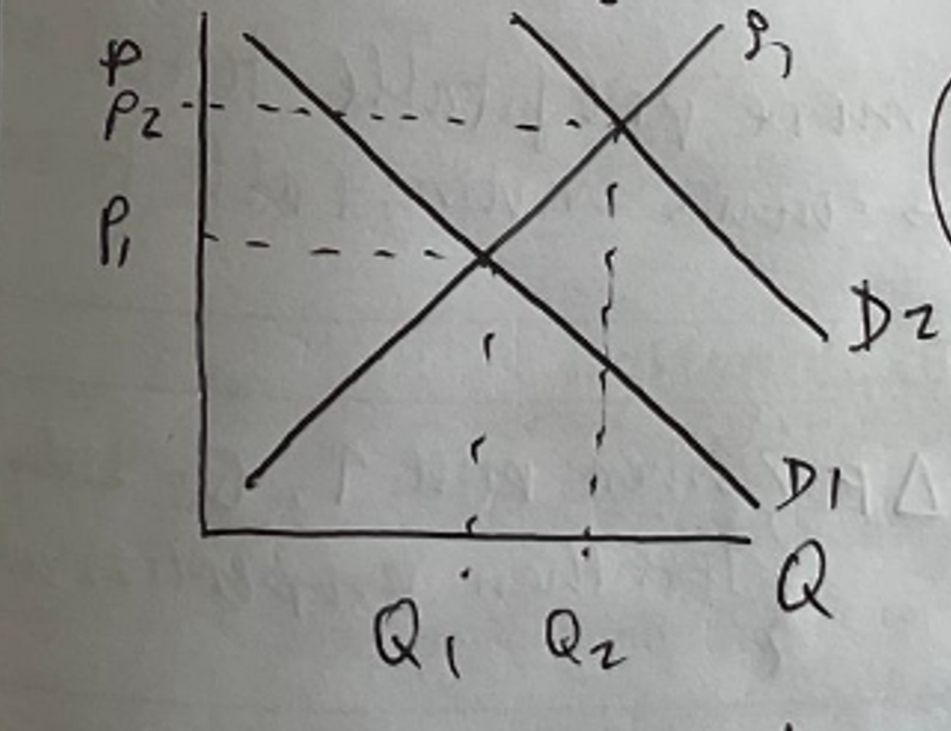
Luxury Good - Increase in income:
Luxury Good - Decrease in income:
-
Luxury goods are Y elastic, meaning as Y (income) increases, QD (quantity demanded) increases more than proportionately.
-
The large shift in demand indicates a big increase in Y which is reflected when price increases.
-
A large shift in demand causes a large increase in price and a large increase in both QD and QS.
-
Shift in Demand to the right → shortage price increases.
-
As Y falls, there will be a large fall in D.
-
As it's Y elastic for luxury goods, Qd and Qs will decrease more than proportionately.
-
Large decrease in P and a large decrease in Qd and Qs.
-
Shift in D to the left leads to surplus and further price drop.
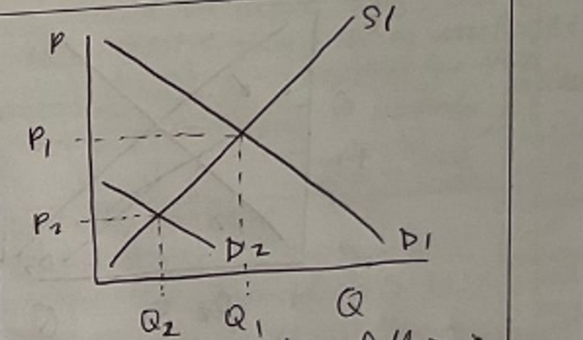
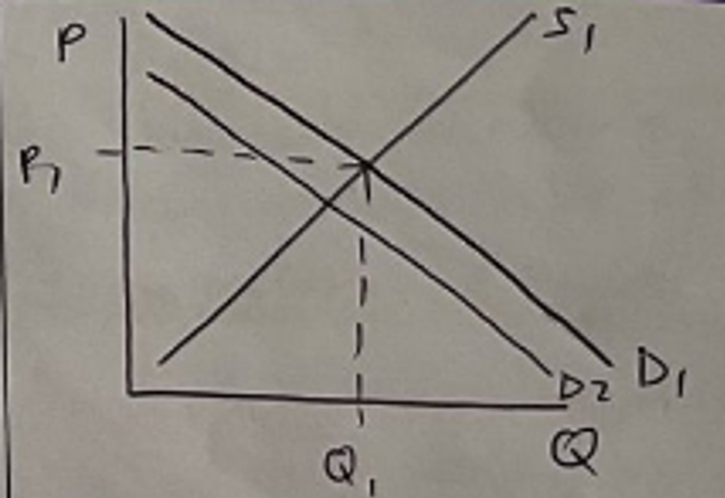
Necessity - Increase in income:
Necessity - Decrease in Y:
-
necessities are income inelastic
-
D1 shifts to D2, causing a small decrease in Qd and Qs, and a small decrease in price.
-
Given an increase in Y, Qd and Qs decrease less than proportionately.
-
Small shortage in supply leads to a small increase in price.
-
A decrease in Y leads to a less than proportionate decrease in Qd.
-
D shifts slightly to the left.
-
A small surplus at P1 leads to a small decrease in price.
-
Overall, there is a small decrease in both Qd and Qs.
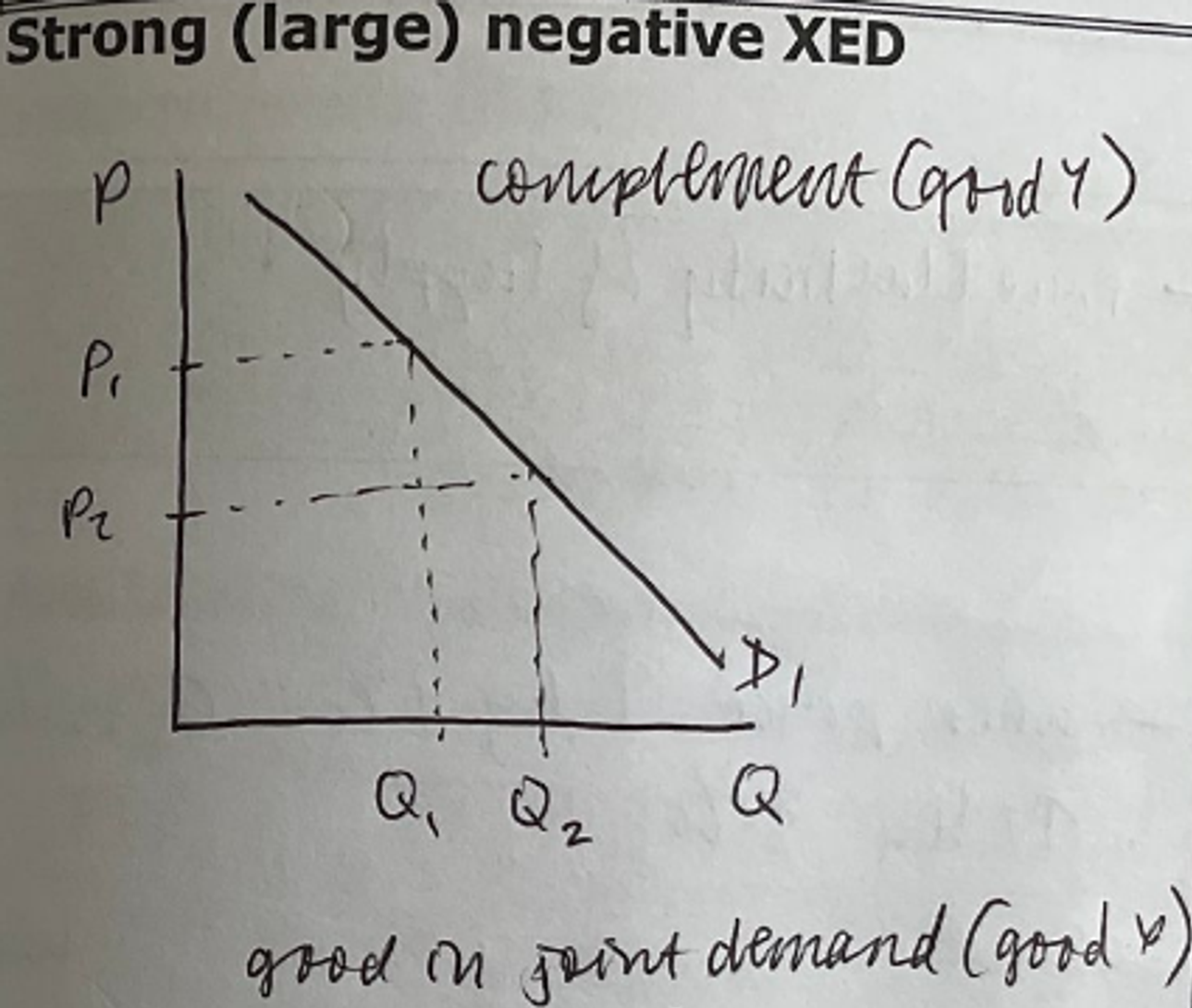
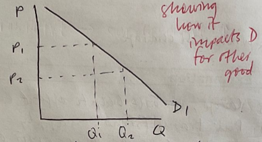
Diagram: Strong (Large) Negative XED (Complementary Good Y)
Diagram: Price of Complement Decreases
- XED is only applicable to price changes.
- SUBS: Large price changes of substitute goods may not affect the related good as predicted by XED due to wasted resources.
- Can only predict changes for small price changes in the related good.
- In cases where products are closely related, XED will accurately predict their response to price changes of related goods.
- The diagram shows the demand curve D1 shifting to D2 as the price of a complementary good decreases from P1 to P2.
- As the price of the complement decreases, the quantity demanded of the good increases from Q1 to Q2.
- The demand curve shifts significantly due to the strong relationship between the complementary goods.
- Price of complement decreases: Many consumers buy it, and as a result, many acquire the complementary good in question.
- Ceteris paribus may not hold: XED may not accurately predict demand changes for goods due to other factors affecting demand/supply (not just price).
- If the price of a substitute increases, the effect on the complementary good's demand might not be as strong due to other influencing factors.
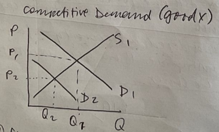
Diagram: Substitute (Good Y)
Diagram: Competitive Demand (Good X)
-
If substitutes decrease in price: The demand for the firm's products will decrease unless they also lower their prices.
-
Substitute (Good Y): Given a decrease in the price of a substitute, where XED (cross-price elasticity of demand) is a large figure, the demand for the competitive good will grow, leading to a decrease in demand for the original product and a decrease in profits.
-
XED high positive:
-
Strong substitutes: Firms would lower prices to gain more market share, expecting a large increase in demand for their product.
-
BAD: If the increase in demand is not as high as expected, firms might have unnecessarily increased capacity (factors of production) and invested in capital goods.
-
Firms consider lowering prices so that the demand for their product increases significantly, which can lead to higher revenue and profits.
-
XED large positive value:
-
Indicates close complements.
-
Suggests firms should adjust prices as an increase in demand is anticipated.
-
Firms may increase capacity to meet higher demand.
-
BUT:
-
If XED is not a large positive value, then the demand might not increase as much as expected, leading to wasted resources in increasing capacity and potentially bad decisions.
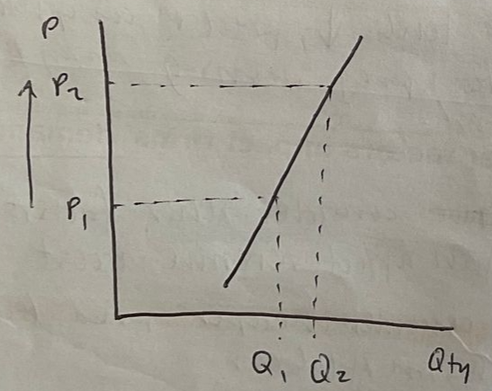
Inelastic Supply
Elastic Supply
Explanation:
Even when prices increase a lot, the quantity supplied increases less than proportionately.
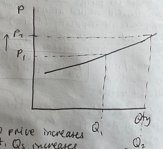
Explanation:
When price increases even slightly, the quantity supplied increases more than proportionately.
2.6.7 Price Elasticity of Demand (PED) and a Firm's Total Revenue
Price Elasticity of Demand (PED) measures the responsiveness of the quantity demanded of a good to a change in its price. It is calculated as the percentage change in quantity demanded divided by the percentage change in price.
Relationship between PED and Total Revenue:
Total Revenue (TR) is calculated as:
The relationship between PED and TR can be categorized into three scenarios:
- Elastic Demand (PED > 1):
- When demand is elastic, a price decrease leads to a proportionally larger increase in quantity demanded.
- This results in an increase in total revenue.
- Conversely, a price increase leads to a proportionally larger decrease in quantity demanded, resulting in a decrease in total revenue.
- Inelastic Demand (PED < 1):
- When demand is inelastic, a price decrease leads to a proportionally smaller increase in quantity demanded.
- This results in a decrease in total revenue.
- Conversely, a price increase leads to a proportionally smaller decrease in quantity demanded, resulting in an increase in total revenue.
- Unitary Elastic Demand (PED = 1):
- When demand is unitary elastic, a change in price leads to a proportionally equal change in quantity demanded.
- This means total revenue remains unchanged when the price changes.
Price elasticity of demand and revenue
Diagram:
To illustrate this, consider a linear demand curve and the corresponding total revenue curve.
Demand Curve:
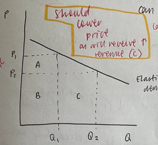
Can calc. revenue →
Can't calc. profit as doesn't show cost curve (CC)
1 way to compare:
- At P1 revenue = A + B
- At P2 revenue = B + C
- (A + B < B + C)
2nd way:
- A+
B<B+C - A < C
C= Gain in revenue from lowering the price and many more customers buying the product
(Q1 → Q2) + P2
A = reveune lost due to decrease in price from P1 to P2
Existing consumer of Q1 paying a lower price where at the price of P1 consumers are willing to buy same for less
Exercise 1:
A cigarette company has an inelastic demand curve. Using a diagram, explain whether the firm should charge a low or a high price.
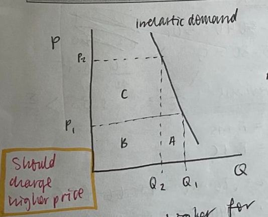
At P1, revenue = A + B
At P2, revenue = B + C
B + C > A + B
C > A
Net change in revenue
C - A = increase in revenue
as  C > A
Revenue is higher for inelastic demand with an increase in price
Gain from existing consumers
A= loss in revenue from Q1- Q2
consumers no longer buying the product
Amount of loss of revenue = (Q1 - Q2) + P1
Key Points:
- Elastic Range: On the demand curve, the upper-left portion (where price is high and quantity is low) represents elastic demand. In this range, lowering the price increases total revenue.
- Inelastic Range: The lower-right portion (where price is low and quantity is high) represents inelastic demand. In this range, raising the price increases total revenue.
- Unitary Elastic Point: The midpoint of the demand curve represents unitary elastic demand. At this point, total revenue is maximized, and any change in price leaves total revenue unchanged.
Conclusion:
Understanding the relationship between PED and total revenue helps firms make pricing decisions. By knowing whether the demand for their product is elastic or inelastic, firms can predict how changes in price will affect their total revenue.

500K+ Students Use These Powerful Tools to Master Elasticity For their A-Level Exams.
Enhance your understanding with flashcards, quizzes, and exams—designed to help you grasp key concepts, reinforce learning, and master any topic with confidence!
120 flashcards
Flashcards on Elasticity
Revise key concepts with interactive flashcards.
Try Economics Flashcards12 quizzes
Quizzes on Elasticity
Test your knowledge with fun and engaging quizzes.
Try Economics Quizzes29 questions
Exam questions on Elasticity
Boost your confidence with real exam questions.
Try Economics Questions27 exams created
Exam Builder on Elasticity
Create custom exams across topics for better practice!
Try Economics exam builder18 papers
Past Papers on Elasticity
Practice past papers to reinforce exam experience.
Try Economics Past PapersOther Revision Notes related to Elasticity you should explore
Discover More Revision Notes Related to Elasticity to Deepen Your Understanding and Improve Your Mastery