6.3.2 Using Exps & Logs in Modelling

Modelling With Exponentials

An exponential relationship is one in which the variable appears in the power. For example:

• $y = 3^x$
• $y = 5e^{7t}$
• $Q = Ae^{kt}$

---

Rearranging the Equation

It's possible to rearrange the equation into the form $y = mx + c$ to obtain a straight line using logarithms.

1. Start with: $P = Ae^{-kt}$
2. Take natural logarithms on both sides: $\ln(P) = \ln(Ae^{-kt})$
3. Use logarithm properties: $\ln(P) = \ln(A) + \ln(e^{-kt})$
4. Simplify: $\ln(P) = \ln(A) - kt$
5. Rearrange: $\ln(P) = -kt + \ln(A)$

This equation is in the form $y = mx + c$ , where:

• $y = \ln(P)$
• $x = t$
• $m = -k$
• $c = \ln(A)$

If you plot $\ln(P)$ on the $y$-axis and $t$ on the $x$-axis, you will get a straight line.

---

Analysing the Relationship Between $R$ and $T$

1. The planet Saturn has many moons. The table below gives the mean radius of orbit and the time taken to complete one orbit, for five of the best-known of them. | Moon | Tethys | Dione | Rhea | Titan | Iaepetus | |---|---|---|---|---|---| | Radius $R$ (x $10^5$ km) | 2.9 | 3.8 | 5.3 | 12.2 | 35.6 | | Period $T$ (days) | 1.9 | 2.7 | 4.5 | 15.9 | 79.3 |

It is believed that the relationship between $R$ and $T$ is of the form $R = kT^n.$

i) Rearranging the Equation

To confirm the relationship, rearrange the equation into a straight-line form, allowing you to plot the graph and verify if it gives a straight line.

Starting with: $R = kT^n$

Take natural logarithms on both sides: $\ln(R) = \ln(kT^n)$

Using logarithm properties: $\ln(R) = \ln(k) + \ln(T^n)$

Further simplification: $\ln(R) = \ln(k) + n\ln(T)$

This is now in the straight-line form $y = mx + c$ , where:

• $y = \ln(R)$
• $x = \ln(T)$
• $m = n$ (the gradient)
• $c = \ln(k)$ (the $y$-intercept)

ii) Plotting the Graph

If we plot $\ln(R)$ against $\ln(T)$, and the original relationship $R = kT^n$ is true, we should get a straight line. The table below gives the values:

$R$	$T$
$2.9 \times 10^5$	1.9
$3.8 \times 10^5$	2.7
$5.8 \times 10^5$	4.5
$12.2 \times 10^5$	15.9
$35.6 \times 10^5$	79.3

By calculating the logarithms and plotting these points, the straightness of the line will confirm the relationship between $R$ and $T$.

Data Points

The table provides the values of $\ln(T)$ and $\ln(R)$:

$\ln(T)$	$\ln(R)$
0.642	12.58
0.995	12.85
1.50	13.10
2.77	14.01
4.37	15.09

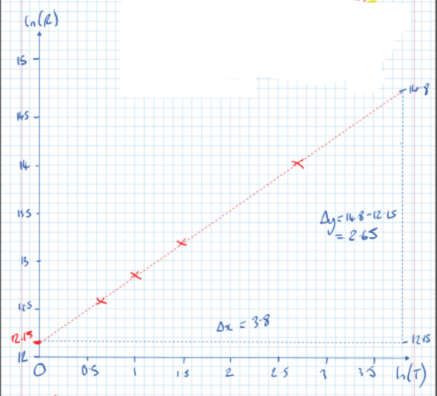
Graph Analysis

• A plot of $\ln(R)$ ($y$-axis) against $\ln(T)$ ($x$-axis) results in a straight line.
• The gradient $m = n$ is calculated from the change in $y$ and $x$: $\Delta y = 15.09 - 12.58 = 2.65$ $\Delta x = 4.37 - 0.642 = 3.8$

Therefore, the gradient $n$:

$n = \frac{\Delta y}{\Delta x} = \frac{2.65}{3.8} \approx :highlight[0.697]$

• The y-intercept is found at $\ln(k) = 12.15$: $k = e^{12.15} \approx :highlight[1.89 \times 10^5]$

Final Equation

The relationship between $R$ and $T$ is confirmed as:

$R = :highlight[1.89 \times 10^5] \times T^{:highlight[0.697]}$

For example, when $R = 1.4 \times 10^5$:

$1.4 \times 10^5 = 1.89 \times 10^5 \times T^{0.697}$

$\frac{1.4 \times 10^5}{1.89 \times 10^5} \approx T^{0.697}$

$0.7407 \approx T^{0.697}$

$T \approx (0.7407)^{\frac{1}{0.697}} \approx :highlight[0.65 days]$

---