Biodiversity Prediction Models (HSC SSCE Biology): Revision Notes
Biodiversity Prediction Models
Introduction to biodiversity prediction models
Scientists use mathematical and computer-based models to predict how biodiversity will change over time. These models help us understand how human activities and environmental changes might affect species populations and ecosystems. By studying patterns from the past and present, we can make informed predictions about the future of biodiversity.
A model is a simplified representation of a complex system that helps us understand and predict real-world phenomena. In ecology, models are essential because ecosystems are too complicated to study completely in their natural environment.
Models allow scientists to input data about species numbers and environmental factors, then calculate likely outcomes based on mathematical relationships. This simplified approach makes it possible to analyze complex ecological interactions that would be impossible to study directly in nature.
Historical foundation: Thomas Malthus and population modelling
Thomas Malthus (1766-1834) was an English scholar who pioneered the use of mathematical models to predict population changes. Although his work focused on human populations, his principles apply to all species. Malthus made several key observations:
- Resources in an environment increase slowly
- Populations have the capacity to grow quickly
- Populations will eventually outgrow their ability to feed themselves
- High fertility leads to competition, which causes starvation, disease and conflict
- These factors reduce population numbers, creating a natural negative feedback loop
Malthus developed the Malthusian growth model (also called the exponential growth model) to show how populations grow when resources are unlimited:
where:
- = initial population size
- = population growth rate
- = time
This work was revolutionary because Malthus was one of the first people to use quantitative data and mathematical modelling to predict future trends. His ideas significantly influenced Charles Darwin's development of the Theory of Evolution by Natural Selection.
Models to predict future population changes
Conservation biologists use population models to assess whether species are vulnerable to extinction. They look for rapid declines in population size, habitat destruction, or species that are endemic to small areas (meaning they only exist in one limited location).
Understanding the past is critical for predicting the future. Environmental management typically uses two complementary approaches:
Equilibrium models
These models establish a baseline from a specific point in the past. In Australia, scientists often use the moment of first European settlement (1788) as the baseline. This represents the state of the environment before major European impacts.
The assumption is that biological communities were relatively stable at the baseline point, existing in a state of equilibrium. This provides a reference point for measuring subsequent changes.
Non-equilibrium models
These models measure changes since the baseline. They factor in disturbances to the ecosystem. A disturbance is any event that removes organisms from a community or changes resource availability. Examples include:
- Natural disturbances: storms, fires, floods, droughts
- Human-caused disturbances: land clearing, overgrazing, pollution
Disturbances can be classified by their intensity:
- High-level disturbances: high frequency or high intensity events
- Low-level disturbances: low frequency or low intensity events
Not All Disturbances Are Negative
It's important to note that not all disturbances are negative. Some disturbances create new opportunities for certain species. Historical mass extinction events, while devastating, often led to increased ecosystem diversity over time as surviving species evolved to fill empty ecological niches.
Approaches to constructing population models
Scientists use two main approaches when building models of biological communities:
Top-down models
These models examine how changes at the top of the food chain affect lower trophic levels.
Top-Down Model Applications
A top-down model might investigate:
- The effect of losing top predators (such as eagles) on populations of smaller predators and herbivores
- How biomagnification of pesticides in predatory birds impacts the entire food web
Bottom-up models
These models examine effects starting from the bottom of the food chain. They predict what happens when producers (plants, algae, certain bacteria) are removed or reduced.
Bottom-Up Model Applications
For example:
- How does a reduction in phytoplankton due to climate change affect zooplankton, filter-feeding invertebrates, and whales?
Population growth models
Scientists recognise three main types of population growth models:
Geometric growth
When the environment is ideal with no limiting factors, populations can grow at a geometric rate. This type of growth is evenly distributed throughout the year. In geometric growth:
- There is a fixed rate of population increase within a given time period
- Population sizes are compared to the previous year at the same time
Geometric Growth Equation
The equation for geometric growth is:
where:
- = geometric growth rate (lambda)
- = time in years
- = initial population size (at time = 0)
- = population size at time
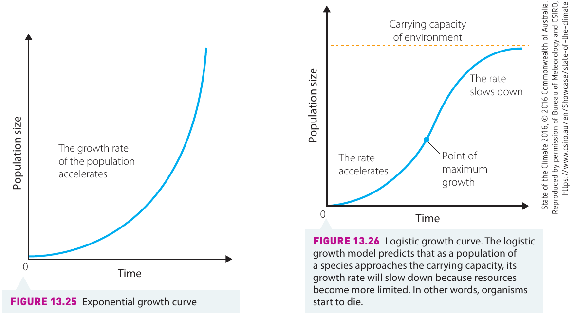
Exponential growth
When growth is intermittent during the year but resources remain unrestricted, the growth rate is exponential. The growth curve has a characteristic J-shape.
Classic Exponential Growth: Bacterial Culture
Bacteria growing in a Petri dish are a classic example of exponential growth. The population accelerates continuously as long as resources are available and waste products don't accumulate to toxic levels.
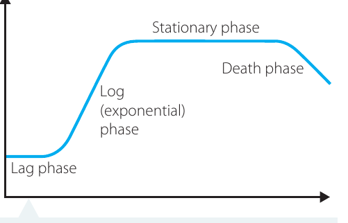
The bacterial growth curve shows four distinct phases:
- Lag phase: initial adaptation period with slow growth
- Log (exponential) phase: rapid population increase
- Stationary phase: growth rate equals death rate
- Death phase: population declines as resources are exhausted
Logistic growth
This is the most common growth pattern in nature. Populations initially grow rapidly, but growth slows as competition for limited resources increases. The graph forms a characteristic sigmoid (S-shaped) curve.
The logistic model introduces the concept of carrying capacity (), which is the largest population size that an ecosystem can support without negative effects.
Carrying capacity is dynamic and changes with:
- Rainfall patterns
- Abundance of resources
- Presence of predators
- Disease prevalence
Logistic growth typically has three distinct phases:
- Acceleration phase: population growth speeds up
- Point of maximum growth: fastest rate of increase
- Deceleration phase: growth rate slows as carrying capacity is approached
Computer modelling in environmental management
Computer models have revolutionised environmental management by allowing scientists to process vast amounts of data and test multiple scenarios. One example is the Western Australian Rangeland Monitoring System (WARMS), which predicts the possible impacts of climate change on ecosystems.
Data Requirements for Computer Modelling
Computer modelling requires numerical data, including:
- Species population counts from field sampling
- Abiotic factors (temperature, rainfall, soil pH, etc.)
- Historical trends over time
By mapping population trends alongside environmental variables, scientists can establish mathematical relationships. For example, they might link a steady rise in atmospheric temperature to specific changes in a species' physical characteristics or behaviour.
Case study: the Australian ringneck parrot

Scientists studying the Australian ringneck parrot (Barnardius zonarius) in Western Australia discovered that the population's average wingspan has been increasing over time. They hypothesised that:
- Increased wing length provides greater surface area for heat loss through skin capillaries
- Birds cannot sweat, so they must lose heat through radiation from their skin
- Rising average temperatures act as a selection pressure favouring birds with longer wings
- Birds that thermoregulate more efficiently have a reproductive advantage
This research was made possible through computer modelling, which allowed scientists to analyse years of data on wing measurements alongside climate data, revealing patterns that would have been difficult to detect otherwise.
Case study: Parramatta River mangroves
The Parramatta River in Sydney provides an important lesson about the accuracy of models and assumptions. For many years, it was assumed that mangroves along the river were remnants of more extensive growth destroyed during European settlement.
However, research by L. C. McLoughlin (1987, 2000) using historical sources revealed the opposite: mangroves were originally confined to small patches in lower areas of the river. Over time, mangrove growth increased, eventually lining all available riverbanks and replacing saltmarshes.
The Critical Lesson of Accurate Data
This incorrect assumption had significantly influenced foreshore planning and restoration activities. The case demonstrates that models are only as accurate as the data they are based on. Using better historical data led to more effective environmental management decisions.
Using models to manage human impacts on future ecosystems
The role of palaeontology
Palaeontology (the study of fossils) provides excellent data for building models to guide future ecosystem management. Fossils are remains of organisms that were uniquely suited to their past environments. They provide invaluable information about what conditions were like in the past.
What Fossil Studies Reveal
Through fossil studies, scientists can:
- Determine how organisms have changed over time
- Understand evolutionary relationships between species
- Investigate why organisms became extinct
- See the effects of extinction on other organisms
- Recognise changes in past distribution patterns
This information helps predict how current species distributions might change in response to environmental pressures.
Interpreting environmental conditions from fossils
Fossils provide clues about the environment in which organisms lived:
Marine environments: Fossils of corals, brachiopods, or echinoderms indicate the rocks were deposited in ocean environments, because living representatives of these groups are only found in the sea today.
Terrestrial environments: Fossils of land-dwelling animals (like kangaroos) indicate deposition on land or in adjacent freshwater bodies.
Tropical shallow seas: Reef-building corals indicate warm, shallow seas (less than 200 m deep) where sunlight could reach the photosynthetic algae living within the coral tissue.
Climate information: The types of plants preserved as fossils indicate whether the climate was tropical, temperate, or arid. For example, finding fossils of rainforest plants in areas that are now desert indicates significant climate change.
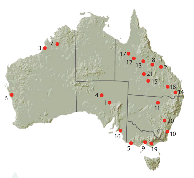
Australian fossil sites and their findings
Australia has many important fossil sites that provide information about past ecosystems. These sites help us understand how environments and species have changed over millions of years.
Key Australian Fossil Sites
Lightning Ridge (110 million years ago): Contains fossils of early monotremes (like Steropodon galmani), echidnas, platypus, and both herbivorous and carnivorous dinosaurs. The environment was forests of ferns and pines with the beginnings of flowering plants.
Murgon (55 million years ago): Shows rainforests after the extinction of dinosaurs. Contains placental mammals, crocodiles, snakes, frogs, salamanders, marsupial mammals, and rainforest plants. This indicates abundant marsupial mammals with few placental mammals.
Koonwarra (115-118 million years ago): A large freshwater lake ecosystem with fish, plants, insects (including mayfly nymphs and fleas), crustaceans, spiders, birds, and crabs.
Riversleigh (25 million-40,000 years ago): Extremely diverse rainforest fauna including parrots, ancestors of emus and cassowaries, many marsupials (kangaroos, possums, wombats), crocodiles, snakes, lizards, turtles, and monotremes.
Wellington Caves (5 million-30,000 years ago): Shows the transition from leaf-browsing to grass-grazing marsupials over time, indicating expansion of grasslands. Contains giant marsupial wombats (Diprotodon) and marsupial lions (Thylacoleo).
Naracoorte (300,000 years ago): Contains megafauna (very large animals) including eastern grey kangaroos, swamp wallabies, and extinct giant marsupials, along with birds, reptiles, and frogs.
Understanding species evolution, survival, and extinction
By studying the fossil record and current species, scientists can propose reasons why species evolved, survived unchanged, or became extinct:
Extinct Species Example - Thylacine (Tasmanian tiger)
Multiple factors likely contributed to extinction:
- Introduction of dingoes 3,500 years ago created new competition
- Hunting by farmers who saw them as threats to livestock
- Government bounty programs encouraged killing
- Disease may have contributed
- Likely a combination of all these factors in succession
Extinct Species Example - Diprotodon optatum (giant marsupial)
Probable causes of extinction:
- Human hunting after people arrived in Australia
- Climate change affecting food sources
- Possibly a combination of both factors
Survived Species Example - Spotted cuscus
Successful survival strategies:
- Retreated with the rainforest as climate changed
- Could adapt to changing habitat distribution
Evolved Species Example - Kangaroos (Macropus species)
Successful adaptations to environmental changes (forests to grasslands):
- Reduced number of toes and developed bipedal hopping for escaping predators in open grassland
- Changed from leaf-browsing diet to grass-grazing diet
- These adaptations gave them advantages in the increasingly arid Australian environment
Remember!
Key Points to Remember:
-
Models are essential tools for predicting biodiversity changes and informing conservation decisions
-
Thomas Malthus pioneered population modelling using mathematical equations to show exponential growth when resources are unlimited
-
Three main types of population growth exist: geometric (evenly distributed), exponential (J-shaped curve), and logistic (S-shaped sigmoid curve with carrying capacity)
-
Equilibrium and non-equilibrium models work together: equilibrium models establish baselines from the past, while non-equilibrium models track changes and disturbances since then
-
Computer modelling revolutionised conservation biology by processing large datasets and establishing relationships between environmental variables and species populations
-
Palaeontology provides crucial data for predicting future changes by showing how past environments and species responded to climate change and other pressures
-
Australian fossil sites demonstrate how ecosystems changed from dinosaur-dominated forests to modern grasslands with marsupials, helping predict future responses to environmental change