Long-Run Phillips Curve Revision Notes for HSC SSCE Economics

Long-Run Phillips Curve

Introduction: the original Phillips curve

The Phillips curve demonstrates a fundamental economic challenge: governments cannot easily achieve both low inflation and low unemployment simultaneously. This trade-off emerged as a key policy consideration in the post-Second World War era.

The relationship works through two main channels:

infoNote

Understanding the Trade-off Mechanism

The Phillips curve operates simultaneously in both the goods market and labour market, creating interconnected pressures that link employment levels to price stability.

In the goods market: When economic growth accelerates and creates jobs, it reduces unemployment. However, this stronger growth also generates excessive demand for goods and services, which pushes prices upward.

In the labour market: Economic expansion creates additional demand for workers. This tight labour market drives wages higher. Businesses then increase their prices to maintain profit margins, contributing to overall inflation.

The following diagram illustrates this trade-off:

lightbulbExample

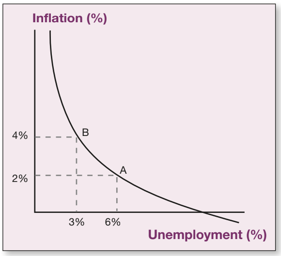
Worked Example: The Original Phillips Curve Trade-off

In this example, expansionary government policies reduce unemployment from $6\%$ to $3\%$ (moving from point A to point B). However, this comes at a cost: inflation rises from $2\%$ to $4\%$ .

Key observation: For every $3$ percentage point reduction in unemployment, inflation increases by $2$ percentage points. This inverse relationship formed the basis of macroeconomic policy thinking for several decades.

The breakdown: stagflation in the 1970s

During the 1970s, this neat theoretical relationship collapsed. In Australia and other industrialised economies, a new phenomenon emerged: stagflation. This occurs when high inflation persists alongside high unemployment and economic stagnation.

Policymakers faced a dilemma. Should they:

Loosen macroeconomic policies to reduce unemployment? (This might worsen inflation)
Tighten macroeconomic policies to combat inflation? (This might increase unemployment)

chatImportant

The Critical Limitation Revealed

The original Phillips curve only accounted for demand-pull inflation (caused by excessive demand in a growing economy). It completely ignored cost-push inflation, which arises from supply-side factors such as oil price shocks. This blind spot meant policymakers lacked the tools to address stagflation effectively.

The persistent stagflation prompted economists to completely rethink the relationship between unemployment and inflation.

The long-run Phillips curve: a new framework

The solution came through developing the Long-Run Phillips Curve, also known as the Friedman-Phelps Expectations Augmented Phillips curve. This refined model incorporates two crucial long-term economic principles that explain why the original Phillips curve failed.

Natural rate of unemployment

The natural rate of unemployment ( $U_n$ ) represents the baseline level of unemployment that exists even in a healthy economy. This includes:

Frictional unemployment: People between jobs
Structural unemployment: Workers whose skills don't match available jobs
Seasonal unemployment: Jobs that vary with seasons
Hard-core unemployment: Those facing significant barriers to employment

chatImportant

A Fundamental Policy Constraint

Demand-management policies and standard macroeconomic tools cannot reduce unemployment below the natural rate. Any attempt to do so triggers inflation without achieving lasting employment gains. This represents a hard limit on what expansionary policies can achieve.

Inflationary expectations

When workers and businesses anticipate higher inflation, they adjust their behaviour accordingly:

Workers demand higher wages to compensate for expected price increases
Businesses raise prices in anticipation of higher costs
These actions create a self-fulfilling prophecy, embedding inflation into the economy

infoNote

The model defines the "long term" as the period needed for inflationary expectations to adjust fully to actual inflation levels. In practice, this adjustment period typically ranges from several months to a few years, depending on how quickly information spreads through the economy.

How the model works: a step-by-step analysis

The following diagram illustrates the complete Friedman-Phelps framework:

lightbulbExample

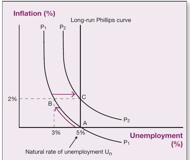
Worked Example: The Complete Adjustment Process

Consider an economy starting at point A, where:

Unemployment equals the natural rate ( $5\%$ )
Inflation stands at $0\%$
The economy sits on short-run Phillips curve $P_1$

Stage 1: Expansionary policy (A to B)

The government implements expansionary macroeconomic policy, perhaps through increased government spending. The economy moves to point B:

Unemployment falls to $3\%$ (below the natural rate)
Inflation rises to $2\%$
This appears to demonstrate the traditional Phillips curve trade-off

Stage 2: Adjustment period (B to C)

However, this success proves temporary. Workers gradually realise that inflation now runs at $2\%$ . They respond by demanding higher wages to maintain their real purchasing power.

Businesses face a dual pressure:

Higher wage costs from worker demands
Recognition that prices across the economy have risen by $2\%$

In response, businesses reduce production and cut their workforce. Unemployment begins creeping back toward the natural rate.

Stage 3: New equilibrium (point C)

Eventually, the economy reaches point C:

Unemployment returns to $5\%$ (the natural rate)
Inflation remains at $2\%$
Inflationary expectations have adjusted upward
The economy has shifted to a new short-run Phillips curve ( $P_2$ )

chatImportant

Critical insight: The expansionary policy achieved no long-term reduction in unemployment. Its only lasting effect was permanently higher inflation.

The long-run Phillips curve appears as a vertical line at the natural rate of unemployment ( $U_n$ ). This vertical line demonstrates that expansionary policy cannot reduce unemployment below the natural rate in the long term.

Hysteresis: the asymmetric danger

The model becomes more complex when considering contractionary policies. In theory, tight macroeconomic policies should reverse the process:

Move the economy down and right along a short-run Phillips curve
Reduce inflation while temporarily increasing unemployment
Eventually return to the natural rate with lower inflation

However, real-world experience reveals a problematic phenomenon called hysteresis. This occurs when temporarily higher unemployment becomes permanent.

The hysteresis mechanism

infoNote

Understanding the Hysteresis Process

When contractionary policies increase unemployment, the cyclically unemployed face serious challenges that prevent them from returning to work even after economic conditions improve. This transforms what should be temporary unemployment into a permanent increase in the natural rate itself.

When contractionary policies increase unemployment, the cyclically unemployed face serious challenges:

Loss of job-specific skills through disuse
Deterioration of professional networks and contacts
Declining motivation and confidence
Growing gaps in employment history

These factors transform cyclical unemployment into structural unemployment. Even when economic conditions improve, these workers struggle to find employment. The natural rate of unemployment itself increases.

chatImportant

The Asymmetric Risk

Graphically, hysteresis appears as a rightward shift of the long-run Phillips curve. This creates an asymmetry: expansionary policies raise inflation without reducing unemployment long-term, while contractionary policies may increase unemployment without achieving lasting inflation reductions. Policymakers face a "heads I lose, tails I lose" scenario.

Policy implications: five key lessons

The Friedman-Phelps analysis fundamentally changed macroeconomic policy thinking:

1. Expansionary policy cannot reduce long-term unemployment

Using fiscal or monetary stimulus to push unemployment below the natural rate proves futile. The economy eventually returns to the natural rate, leaving only higher inflation as the permanent legacy.

2. Expansionary policy only increases long-term inflation

The sole permanent effect of expansionary macroeconomic policy is higher inflation. Any employment gains prove temporary as inflationary expectations adjust.

3. Contractionary policy may permanently increase unemployment

Through hysteresis, attempts to reduce inflation by increasing unemployment can backfire, raising the natural rate itself. This makes contractionary policy particularly dangerous.

4. Long-term unemployment reduction requires supply-side policies

To genuinely lower unemployment, governments must use:

Microeconomic policies: Labour market reforms, education and training programmes
Supply-side policies: Measures that increase the economy's productive capacity
Structural reforms: Changes to tax, welfare, and regulatory systems

5. Managing inflationary expectations matters critically

Keeping inflation expectations anchored prevents the wage-price spiral that drives unemployment back to the natural rate.

These lessons led policymakers to prioritise inflation control while pursuing unemployment reduction through long-term structural measures.

Australian policy applications

Australia's current policy framework reflects these theoretical insights through a carefully balanced approach that addresses both inflation and unemployment without falling into the Phillips curve trap.

Monetary policy: inflation-focused

infoNote

The RBA's Primary Mandate

The Reserve Bank of Australia (RBA) makes monetary policy (setting interest rates) its primary macroeconomic tool. This reflects the lesson that demand-side policies are most effective for managing inflation rather than unemployment.

The RBA's approach includes:

Primary focus: Fighting inflation first
Inflation target band: $2-3\%$ annual inflation, anchoring expectations
Labour market monitoring: Close attention to signs of excessive demand that might trigger wage-price spirals
NAIRU awareness: Though not explicitly calculated, the RBA watches for the non-accelerating inflation rate of unemployment

Fiscal policy: supporting role

Fiscal policy plays a secondary role in demand management:

Provides targeted support during economic slowdowns (e.g., 2009 Global Financial Crisis, 2020 COVID-19 pandemic)
Used strategically to prevent unemployment spikes during crises
Generally maintains a disciplined approach outside crisis periods

Microeconomic policies: long-term unemployment strategy

infoNote

Addressing the Natural Rate Directly

Following the Phillips curve insights, Australia pursues low unemployment not through demand stimulus, but through policies designed to reduce the natural rate itself. This approach avoids the inflationary trap while achieving genuine, sustainable employment gains.

Australia's structural approach includes:

Training and education policies: Building workforce skills to reduce structural unemployment
Tax and welfare reform: Increasing work incentives to reduce voluntary unemployment
Market-oriented reforms: Promoting competition and efficiency throughout the economy
Labour market flexibility: Enabling faster adjustment to economic changes

This multi-pronged approach recognises that sustainable employment gains require structural improvements rather than demand stimulus alone.

bookmarkSummary

Key Takeaways

The original Phillips curve suggested a simple trade-off between unemployment and inflation, but this relationship broke down during 1970s stagflation
The long-run Phillips curve is vertical at the natural rate of unemployment, showing that expansionary policy cannot reduce unemployment long-term
Inflationary expectations cause the economy to return to the natural rate, with only higher inflation remaining as the legacy of expansionary policy
Hysteresis means contractionary policies carry the risk of permanently increasing unemployment, creating an asymmetric problem for policymakers
Effective unemployment reduction requires supply-side and microeconomic reforms, not just demand-management policies
Australia's policy mix reflects these lessons: monetary policy targets inflation, while microeconomic reforms address structural unemployment

Long-Run Phillips Curve (HSC SSCE Economics): Revision Notes