The Log Transformation Revision Notes for VCE SSCE General Mathematics

The Log Transformation

Introduction to logarithmic transformations

When working with bivariate data, you may encounter relationships that are clearly not linear. In such cases, a logarithmic transformation can help straighten out curved patterns, making it possible to fit a linear regression model. This technique builds on the idea you learned earlier about transforming skewed distributions to make them more symmetric.

The logarithmic transformation works by compressing the scale at one end of either the $x$ -axis or the $y$ -axis. This compression can linearise certain types of non-linear associations, allowing you to use the powerful tools of linear regression analysis.

Notation convention

infoNote

Throughout this topic, we follow the standard mathematical convention where $\log x$ means $\log_{10} x$ . This is the logarithm to base 10, which is the default when no base is specified.

Understanding the two types of log transformations

There are two main ways to apply logarithmic transformations to bivariate data, depending on which variable shows the non-linear pattern.

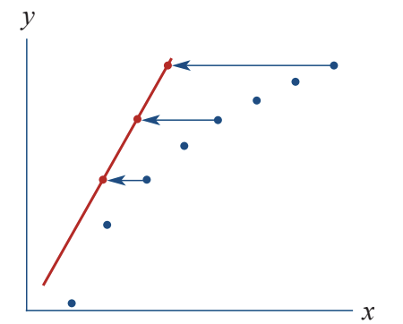
The $\log_{10} x$ transformation

This transformation is applied to the explanatory variable (the $x$ -values). It compresses the higher $x$ -values relative to the lower $x$ -values, whilst leaving the $y$ -values completely unchanged.

Effect: This transformation straightens out curves where the $x$ -variable increases rapidly whilst the $y$ -variable increases more steadily. It's particularly useful when dealing with variables like income, population, or GDP, which can span several orders of magnitude.

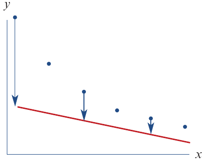
The $\log_{10} y$ transformation

This transformation is applied to the response variable (the $y$ -values). It compresses larger $y$ -values relative to smaller $y$ -values, whilst leaving the $x$ -values unchanged.

Effect: This transformation straightens out curves where the $y$ -variable increases exponentially whilst the $x$ -variable increases linearly. It's particularly useful for data showing exponential growth, such as population growth, disease spread, or compound interest.

Worked example: applying the $\log x$ transformation

Let's examine a real-world example involving the relationship between a country's wealth and the lifespan of its citizens. This example demonstrates how to transform non-linear data into a linear form.

The problem

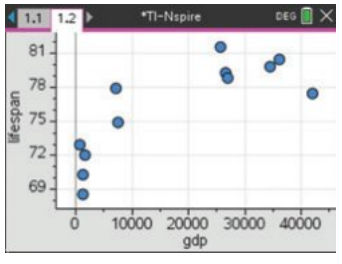
The general wealth of a country, measured by its Gross Domestic Product (GDP) per person, is associated with lifespan. However, this relationship is not linear, as shown in the scatterplot below.

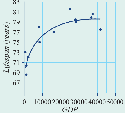
The scatterplot reveals a strong positive association, but the relationship curves rather than forming a straight line. Countries with low GDP show rapid increases in lifespan as GDP increases, but this effect levels off at higher GDP values.

Data table

Here is the data for 12 different countries:

Lifespan (years)	GDP ($)
80.4	36,032
79.8	34,484
79.2	26,664
77.4	41,890
78.8	26,893
81.5	25,592
74.9	7,454
72.0	1,713
77.9	7,073
70.3	1,192
73.0	631
68.6	1,302

Part a: transforming the data and fitting a regression line

lightbulbExample

Worked Example: Transforming GDP Data

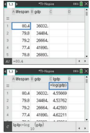
To linearise this relationship, we apply the $\log x$ transformation to the GDP variable. This means we replace each GDP value with its logarithm (base 10).

Steps:

Create a new variable: $\log(\text{GDP})$
Calculate $\log(\text{GDP})$ for each data point
Plot lifespan against $\log(\text{GDP})$
Fit a least squares regression line to the transformed data

After applying the transformation, the scatterplot shows a clear linear relationship:

infoNote

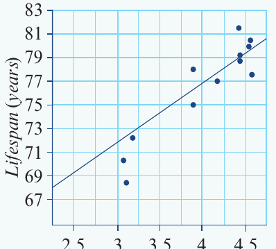
On this transformed plot, when $\log(\text{GDP}) = 4$ , the actual GDP is $10^4 = `$ 10,000$`. The logarithmic scale compresses the large GDP values, spreading out the data points more evenly.

The regression equation:

Using least squares regression on the transformed data, we obtain:

$\text{lifespan} = 54.3 + 5.59 \times \log(\text{GDP})$

This equation models the linear relationship between lifespan and the logarithm of GDP.

Part b: making predictions

lightbulbExample

Worked Example: Predicting Lifespan from GDP

To predict the lifespan in a country with a GDP of $20,000 per person, we substitute this value into our regression equation.

Working:

$\text{lifespan} = 54.3 + 5.59 \times \log(20000)$

Calculate $\log(20000)$ using your calculator:

$\log(20000) = 4.301$

Substitute this value:

\begin{aligned} \text{lifespan} &= 54.3 + 5.59 \times 4.301 \\ &= 54.3 + 24.04 \\ &= 78.3 \text{ years} \end{aligned}

Answer: The predicted lifespan is 78.3 years (to one decimal place).

Worked example: applying the $\log y$ transformation

Now let's look at an example where we need to transform the response variable instead of the explanatory variable.

The problem

During an outbreak of a highly infectious disease, the number of cases was recorded over a 12-day period. The relationship between days and cases is non-linear, showing exponential growth.

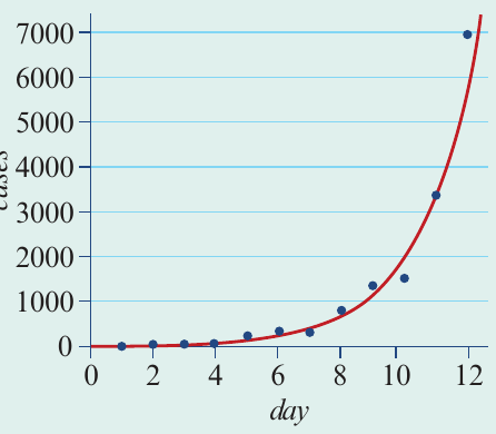
The scatterplot shows a strong positive association, but the number of cases increases exponentially over time. A straight line would not fit this data well.

Part a: transforming the data and fitting a regression line

lightbulbExample

Worked Example: Transforming Disease Case Data

To linearise this exponential relationship, we apply the $\log y$ transformation to the number of cases.

Steps:

Create a new variable: $\log(\text{cases})$
Calculate $\log(\text{cases})$ for each data point
Plot $\log(\text{cases})$ against day
Fit a least squares regression line to the transformed data

After applying the transformation, the relationship becomes linear. The data points now follow a straight line pattern.

infoNote

On the transformed plot, when $\log(\text{cases}) = 3$ , the actual number of cases is $10^3 = 1,000$ . This transformation has compressed the rapidly growing case numbers into a linear pattern.

The regression equation:

Using least squares regression on the transformed data, we obtain:

$\log(\text{cases}) = 1.046 + 0.227 \times \text{day}$

chatImportant

Notice that this equation predicts the logarithm of the number of cases, not the actual number of cases.

Part b: making predictions and converting back

lightbulbExample

Worked Example: Predicting Disease Cases and Converting Back

To predict the number of cases on day 13, we substitute this value into our regression equation. However, we must remember to convert our answer back from the logarithmic scale.

Working:

First, find the predicted logarithm of cases:

\begin{aligned} \log(\text{cases}) &= 1.046 + 0.227 \times 13 \\ &= 1.046 + 2.951 \\ &= 3.997 \end{aligned}

Now we need to find the actual number of cases. Since $\log(\text{cases}) = 3.997$ , we use the inverse operation to find cases:

$\text{cases} = 10^{3.997}$

Use your calculator to evaluate:

$\text{cases} = 9,931$

Answer: The predicted number of cases on day 13 is 9,931 cases (to the nearest whole number).

chatImportant

Key point: When you transform the $y$ -variable using a logarithm, you must always remember to convert your prediction back to the original scale using the exponential function ( $10^x$ ).

Using technology for log transformations

Modern calculators can perform logarithmic transformations and fit regression lines efficiently. Here's a general approach using statistical software or a graphics calculator:

General steps for $\log x$ transformation

Step 1: Enter your data into lists or columns

Create one list for the response variable (e.g., lifespan)
Create one list for the explanatory variable (e.g., GDP)

Step 2: Create a transformed variable

Add a new column for the transformed data
Use the formula: $= \log(\text{explanatory variable})$
The calculator will compute the logarithm for each value

Step 3: Create a scatterplot

Plot the response variable against the transformed explanatory variable
Check that the relationship now appears linear

Step 4: Fit a regression line

Use the calculator's linear regression function
The calculator will provide the equation: $y = a + bx$
Remember: the $x$ in this equation represents the transformed variable $\log(\text{GDP})$

infoNote

Step 5: Write the equation correctly

Always express your final equation using the original variable names:

$\text{lifespan} = 54.3 + 5.59 \times \log(\text{GDP})$

Not simply: $y = 54.3 + 5.59x$

Step 6: Make predictions

Substitute the value of the original explanatory variable (not its logarithm) into your equation, and let the calculator handle the logarithm calculation.

Choosing which transformation to use

When you encounter non-linear data, how do you decide whether to use $\log x$ or $\log y$ ?

Use $\log x$ transformation when:

The $x$ -values span a large range (several orders of magnitude)
The curve shows rapid increase at low $x$ -values, then levels off
The relationship looks like a logarithmic growth pattern
Examples: GDP and lifespan, income and spending on luxuries

Use $\log y$ transformation when:

The $y$ -values increase exponentially
The curve shows slow growth initially, then rapid acceleration
The relationship looks like exponential growth
Examples: disease spread, population growth, compound interest

chatImportant

Exam tip: Always plot your data first. The shape of the scatterplot will guide you in choosing the appropriate transformation.

Important points to remember

When working with logarithms:

infoNote

$\log x$ always means $\log_{10} x$ unless stated otherwise
$\log(10) = 1$ , $\log(100) = 2$ , $\log(1000) = 3$ , etc.
To reverse a logarithm: if $\log(y) = 3.5$ , then $y = 10^{3.5}$

When writing equations:

chatImportant

Always use the original variable names, not just $x$ and $y$
Make it clear which variable has been transformed
Example: $\text{lifespan} = 54.3 + 5.59 \times \log(\text{GDP})$ is correct

When making predictions:

If you transformed $x$ : substitute the original $x$ -value and let the equation calculate the logarithm
If you transformed $y$ : your equation gives $\log(y)$ , so you must use $10^{\text{result}}$ to find $y$

Common mistakes to avoid:

chatImportant

Forgetting to convert back from log scale when using $\log y$ transformation
Using the wrong variable in predictions
Not specifying which variable was transformed in your final equation

Remember!

bookmarkSummary

Key Points to Remember:

Logarithmic transformations compress scales, making non-linear relationships linear by squashing larger values relative to smaller ones.
Two types of transformation: $\log x$ affects the horizontal axis (explanatory variable), whilst $\log y$ affects the vertical axis (response variable).
After transformation, you can use standard linear regression techniques to model the relationship and make predictions.
Always convert back when using $\log y$ transformation: your regression equation gives you $\log(y)$ , so calculate $y = 10^{\text{predicted value}}$ to get the actual prediction.
Use technology wisely: calculators can handle the calculations, but you must understand which variable to transform and how to interpret the results correctly.

The Log Transformation (VCE SSCE General Mathematics): Revision Notes