Modelling Linear Growth and Decay Revision Notes for VCE SSCE General Mathematics

Modelling Linear Growth and Decay

Understanding linear growth and decay

When we talk about linear growth, we mean a situation where a quantity increases by the same fixed amount over equal time periods. Imagine you have $300 in your savings account and you add $20 every week - this represents linear growth because you're adding the same amount each time.

Linear decay works in the opposite way. This occurs when a quantity decreases by the same fixed amount over equal time periods. A common example is when a new car loses a constant amount of value each year.

infoNote

The key characteristic of both linear growth and decay is the constant change - the amount added or subtracted remains the same at every step. This is what makes them "linear" - if you graph these sequences, the points form a straight-line pattern.

The recurrence model for linear growth and decay

We can model both linear growth and decay using recurrence relations. These are mathematical rules that tell us how to get from one term in a sequence to the next.

General forms

Consider these two recurrence relations:

$P_0 = 20, P_{n+1} = P_n + 2$
$Q_0 = 20, Q_{n+1} = Q_n - 2$

The first relation generates a sequence with a linear growth pattern: 20, 22, 24, ...

The second generates a sequence with a linear decay pattern: 20, 18, 16, ...

The common difference

chatImportant

The key feature of linear growth and decay is the common difference, which we represent as $D$ . This is the constant amount we add or subtract at each step.

For any positive constant $D$ :

$V_{n+1} = V_n + D$ models linear growth
$V_{n+1} = V_n - D$ models linear decay

Graphing sequences

When we graph these sequences, we plot individual points (don't join them with lines). The pattern of the dots tells us about the sequence:

An upward slope indicates growth
A downward slope indicates decay

Graphing linear sequences

Let's look at how to graph the terms of a linear sequence.

lightbulbExample

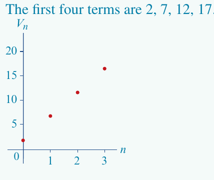
Worked Example: Growth Sequence

For the recurrence relation $V_0 = 2, V_{n+1} = V_n + 5$ :

Starting value: 2
Rule: add 5
First four terms: 2, 7, 12, 17

lightbulbExample

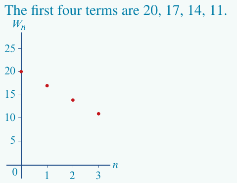
Worked Example: Decay Sequence

For the recurrence relation $W_0 = 20, W_{n+1} = W_n - 3$ :

Starting value: 20
Rule: subtract 3
First four terms: 20, 17, 14, 11

Simple interest investments and loans

Simple interest is a practical application of linear growth. When you invest money or take out a loan with simple interest, the amount grows by the same fixed amount each year.

Key terms

Principal: The initial amount of money borrowed or invested
Interest: The amount added at each step, calculated as a percentage of the principal
Interest rate ( $r\%$ ): The annual percentage rate used to calculate the interest

The simple interest model

Let $V_n$ be the value of the loan or investment after $n$ years, and $r$ be the annual percentage interest rate.

The recurrence relation is:

$V_0 = \text{principal}, \quad V_{n+1} = V_n + D$

where $D = \frac{r}{100} \times V_0$

chatImportant

Notice that $D$ is calculated once, using the original principal, and remains constant throughout. This is what makes simple interest a linear growth model - the interest amount never changes.

Worked example: Setting up a simple interest model

lightbulbExample

Worked Example: Setting Up a Simple Interest Model

Problem: Cheryl invests $5000 in an account that pays 4.8% per annum simple interest. Create a recurrence relation to model this investment.

Solution:

$V_0 = 5000$ (the principal)
$r = 4.8$
$D = \frac{4.8}{100} \times 5000 = 240$
Therefore: $V_0 = 5000, V_{n+1} = V_n + 240$

Using the model to analyse investments

Once we have a recurrence relation, we can use it to answer questions about the investment.

lightbulbExample

Worked Example: Analysing Investments

Using Cheryl's investment model $V_0 = 5000, V_{n+1} = V_n + 240$ :

Part a: Show that the value after 3 years is $5720.

Calculate each term:

$V_0 = 5000$
$V_1 = 5000 + 240 = 5240$
$V_2 = 5240 + 240 = 5480$
$V_3 = 5480 + 240 = 5720$

After three years, the investment is worth $5720.

Part b: When will the investment first exceed $6000?

Using a calculator, we can repeatedly add 240.

The investment first exceeds $6000 after 5 years, when it reaches $6200.

Depreciation

Depreciation refers to the decrease in value of an asset over time. This is particularly important for businesses tracking the value of equipment, vehicles, and other assets.

Important concepts

Future value: The estimated value of an asset at a particular point in time
Scrap value: The value at which an item is no longer useful and will be sold or disposed of

We'll look at two methods of calculating depreciation: flat rate and unit cost.

Flat rate depreciation

With flat rate depreciation, an asset loses a constant amount of value each time period. This amount is typically calculated as a percentage of the original purchase price.

The flat rate depreciation model

Let $V_n$ be the value of the asset after $n$ years, and $r$ be the percentage depreciation rate.

The recurrence relation is:

$V_0 = \text{initial value}, \quad V_{n+1} = V_n - D$

where $D = \frac{r}{100} \times V_0$

infoNote

Notice the similarity to simple interest - the only difference is that we're subtracting $D$ instead of adding it. This makes flat rate depreciation a linear decay model.

Worked example: Modelling flat rate depreciation

lightbulbExample

Worked Example: Modelling Flat Rate Depreciation

Problem: A new car was purchased for $24,000 in 2014. The car depreciates by 20% of its purchase price each year. Create a recurrence relation to model this.

Solution:

$V_0 = 24000$ (initial value)
$r = 20$ (depreciation rate)
$D = \frac{20}{100} \times 24000 = 4800$
Therefore: $V_0 = 24000, V_{n+1} = V_n - 4800$

Analysing flat rate depreciation

lightbulbExample

Worked Example: Analysing Flat Rate Depreciation

Using the car depreciation model $V_0 = 24000, V_{n+1} = V_n - 4800$ :

Part a: Find the value after 2 years.

$V_0 = 24000$
$V_1 = 24000 - 4800 = 19200$
$V_2 = 19200 - 4800 = 14400$

After 2 years, the car is worth $14,400.

Part b: If purchased in 2023, when will the car's value reach zero?

Continuing the pattern:

$V_3 = 14400 - 4800 = 9600$
$V_4 = 9600 - 4800 = 4800$
$V_5 = 4800 - 4800 = 0$

The car reaches zero value in 2028 (after 5 years).

Part c: What was the percentage depreciation rate?

$\frac{4800}{24000} \times 100\% = 20\%$

Unit cost depreciation

Some assets lose value based on how often they're used rather than how much time has passed. For example, a photocopier that has printed thousands of pages is worth less than an unused one of the same age.

The unit cost depreciation model

Let $V_n$ be the value of the asset after $n$ units of use, and $D$ be the cost per unit of use.

The recurrence relation is:

$V_0 = \text{initial value}, \quad V_{n+1} = V_n - D$

infoNote

Note that here, $D$ is simply the depreciation amount per use, not calculated from a percentage. This makes unit cost depreciation particularly useful for equipment where wear and tear depends on usage.

Worked example: Modelling unit cost depreciation

lightbulbExample

Worked Example: Modelling Unit Cost Depreciation

Problem: A professional gardener purchased a lawn mower for $270. The mower depreciates by $3.50 each time it is used.

Part a: Create a recurrence relation.

Solution:

$V_0 = 270$ (initial value)
$D = 3.50$ (depreciation per use)
Therefore: $V_0 = 270, V_{n+1} = V_n - 3.50$

Part b: Find the value after three uses.

$V_0 = 270$
$V_1 = 270 - 3.50 = 266.50$
$V_2 = 266.50 - 3.50 = 263.00$
$V_3 = 263.00 - 3.50 = 259.50$

After three uses, the mower is worth $259.50.

Part c: How many uses until the value is first less than $250?

Continuing:

$V_4 = 259.50 - 3.50 = 256.00$
$V_5 = 256.00 - 3.50 = 252.50$
$V_6 = 252.50 - 3.50 = 249.00$

After six uses, the value first falls below $250.

bookmarkSummary

Key Points to Remember:

Linear growth occurs when a quantity increases by a constant amount ( $V_{n+1} = V_n + D$ ), while linear decay occurs when it decreases by a constant amount ( $V_{n+1} = V_n - D$ )
The constant amount added or subtracted is called the common difference ( $D$ )
Simple interest uses linear growth where $D = \frac{r}{100} \times V_0$ , with the interest calculated on the original principal
Flat rate depreciation uses linear decay where $D = \frac{r}{100} \times V_0$ , with depreciation calculated as a percentage of the original purchase price
Unit cost depreciation uses linear decay where $D$ is the fixed depreciation amount per use, based on usage rather than time
When graphing sequences, plot individual points without joining them - an upward slope indicates growth, a downward slope indicates decay

Modelling Linear Growth and Decay (VCE SSCE General Mathematics): Revision Notes