Rectangular Hyperbolas (VCE SSCE Mathematical Methods): Revision Notes
Rectangular Hyperbolas
Introduction to rectangular hyperbolas
A rectangular hyperbola is a special type of curve that follows the rule:
This function is undefined when , meaning there is no point on the graph where . This is a fundamental property that shapes the entire behavior of the curve.
Table of values
To understand the shape of this curve, we can create a table showing how changes as varies:
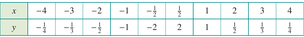
Notice that:
- As gets larger (positively or negatively), gets smaller
- When is positive, is positive
- When is negative, is negative
- There is no value of that produces
These patterns reveal the fundamental relationship between and in a rectangular hyperbola: they are inversely proportional. As one increases, the other decreases in a specific mathematical relationship.
Graph of the basic rectangular hyperbola
When we plot these points and connect them smoothly, we get a distinctive curve with two separate branches:
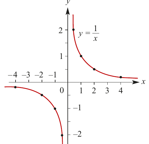
The graph has two separate parts, one in the first quadrant (top right) and one in the third quadrant (bottom left). These branches never meet and never touch the axes.
The symmetry of the rectangular hyperbola is particularly elegant: if you rotate the graph 180° around the origin, it looks exactly the same. This is known as point symmetry about the origin.
Asymptotes
Asymptotes are lines that the curve approaches but never actually touches or crosses. Every rectangular hyperbola has two asymptotes that help define its shape.
Horizontal asymptote
Looking at the graph, we can see that as gets very large (in either direction), the value of gets closer and closer to zero. We write this using special notation:
- As , (read as: "as approaches infinity, approaches from the positive side")
- As , (read as: "as approaches negative infinity, approaches from the negative side")
The curve approaches the -axis (the line ) but never crosses it. Therefore, the line is called a horizontal asymptote.
Think of asymptotes as invisible boundaries that guide the curve's behavior. No matter how far you extend the curve, it will forever approach but never reach these lines.
Vertical asymptote
Similarly, as approaches zero from either direction, the magnitude of becomes extremely large. We write this as:
- As , (read as: "as approaches zero from the positive side, approaches infinity")
- As , (read as: "as approaches zero from the negative side, approaches negative infinity")
The curve approaches the -axis (the line ) but never crosses it. Therefore, the line is called a vertical asymptote.
Transformations of rectangular hyperbolas
Dilations from an axis
When we multiply the basic function by a constant, we create a dilation (stretch) of the graph. The diagram below shows three related hyperbolas:
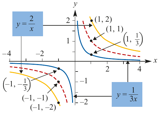
The graphs of and have the same basic shape and the same asymptotes ( and ) as , but they are stretched vertically by different amounts.
Dilation Transformation
The transformation from to is called a dilation of factor from the -axis.
Under this transformation:
- The point on moves to the point on
- The -value doubles while the -value stays the same
Reflection in the x-axis
When we multiply the function by , we reflect the graph in the -axis:
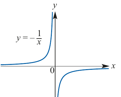
The graph of is the reflection of in the -axis. Notice that:
- The asymptotes remain the same: and
- The branches now appear in the second and fourth quadrants instead of the first and third
- Similarly, is the reflection of in the -axis
Exam tip: Reflecting in the -axis produces the same result for these graphs because of their symmetry. This is a useful property to remember when analyzing transformations.
Translations
We can shift (translate) the graph horizontally and vertically by adding constants. Consider the function:
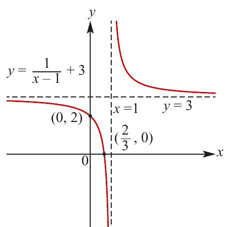
This represents the basic graph translated:
- unit to the right
- units upward
Finding the new asymptotes:
When a rectangular hyperbola is translated, its asymptotes also shift:
- The vertical asymptote moves to
- The horizontal asymptote moves to
The asymptotes shift by the same amount as the graph itself. If you translate the graph units horizontally and units vertically, the vertical asymptote becomes and the horizontal asymptote becomes .
Finding the intercepts:
Unlike the basic hyperbola, translated hyperbolas often cross the axes. To find these intercepts:
For the -intercept, substitute :
So the -intercept is at .
For the -intercept, substitute :
So the -intercept is at .
Sketching rectangular hyperbolas
Using dilations, reflections, and translations, we can sketch any rectangular hyperbola of the form:
Where:
- determines the dilation and orientation (positive or negative)
- determines the horizontal shift
- determines the vertical shift
Worked Example: Sketching
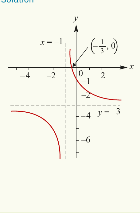
Step 1: Identify the transformations
The basic graph has been:
- Translated unit to the left (because of , which is )
- Translated units downward
Step 2: Find the asymptotes
Vertical asymptote:
Horizontal asymptote:
Step 3: Find the -intercept
When :
The -intercept is .
Step 4: Find the -intercept
When :
The -intercept is .
Worked Example: Sketching
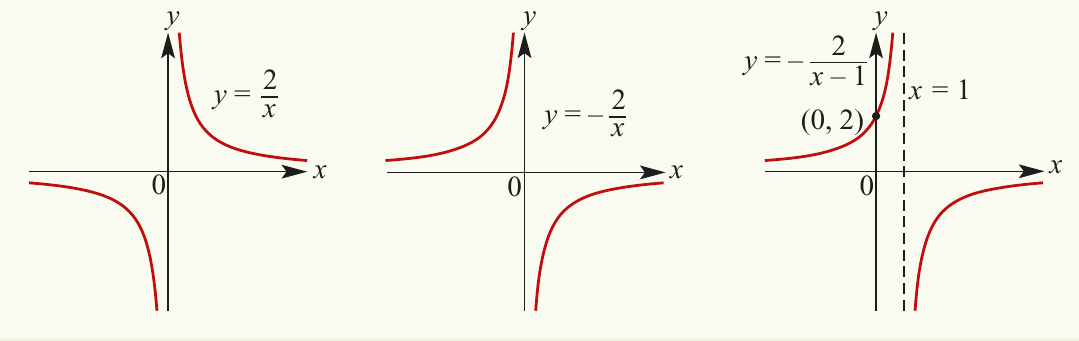
Step 1: Start with the basic graph
Begin with , which has branches in the first and third quadrants.
Step 2: Apply the reflection
Reflect in the -axis to get . This moves the branches to the second and fourth quadrants.
Step 3: Apply the translation
Translate unit to the right to obtain .
Step 4: Identify key features
Vertical asymptote:
Horizontal asymptote:
When :
So the -intercept is at .
Exam tip: When sketching hyperbolas, always mark the asymptotes with dashed lines first, then plot any intercepts, and finally draw the smooth curves in the appropriate quadrants. This systematic approach helps ensure accuracy.
Key Points to Remember:
- A rectangular hyperbola has the form and consists of two separate branches
- The graph has two asymptotes: a vertical asymptote at and a horizontal asymptote at
- The asymptotes are lines that the curve approaches but never touches
- When , the branches lie in opposite quadrants; when , they reflect to different quadrants
- To sketch a hyperbola, first identify the asymptotes, then find any intercepts with the axes, and finally draw the smooth curves