The Truncus (VCE SSCE Mathematical Methods): Revision Notes
The Truncus
Understanding the truncus function
The truncus is a distinctive U-shaped curve that appears when we graph certain reciprocal functions. The most basic form of a truncus comes from the function:
This function creates a symmetrical curve that has some fascinating properties. Unlike many functions you've encountered, this one behaves quite uniquely around the origin and at extreme values.
The truncus has unique properties that make it stand out from other functions you've studied. It's undefined at one point, always produces positive values, and has distinctive behavior at its extremes.
Building the graph from values
To understand how this graph takes shape, let's examine some specific coordinate points. We can calculate y-values for various x-values between -4 and 4:
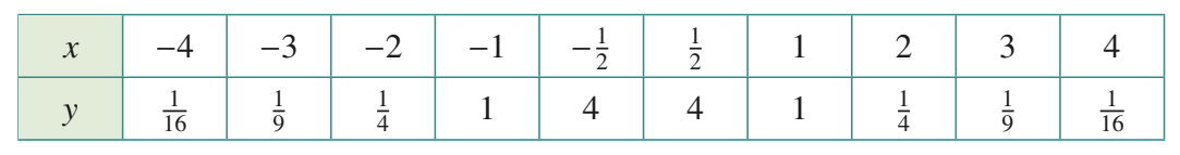
Notice the pattern in these values:
- When , we get
- When , we get
- When , we get
The values are symmetric - the same x-values on opposite sides of zero produce identical y-values. This is because squaring a number always gives a positive result, whether the original number was positive or negative.
When we plot these points and connect them with a smooth curve, we get the characteristic truncus shape:
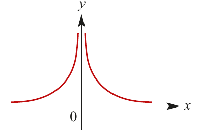
Key features of the truncus
What makes the truncus special
The truncus has several important characteristics that distinguish it from other function graphs. Understanding these features will help you sketch and analyse truncus graphs confidently.
First, the function is undefined at x = 0. We cannot divide by zero, so there is no y-value when x equals zero. This creates a gap in the graph at the origin.
Second, the function only produces positive values. Since we're squaring x in the denominator, the result is always positive (regardless of whether x itself is positive or negative). This means the graph exists entirely above the x-axis.
Asymptotes explained
Understanding Asymptotes
The graph of has two asymptotes - lines that the curve approaches but never actually reaches:
Vertical asymptote: (the y-axis)
As x gets closer and closer to zero from either direction, the y-values grow larger and larger without bound. The curve shoots upward but never crosses or touches the y-axis.
Horizontal asymptote: (the x-axis)
As x gets very large (either positive or negative), the y-values get smaller and smaller, approaching zero. The curve gets closer and closer to the x-axis but never actually touches it.
Behaviour at extreme values
Understanding how the function behaves as x approaches different values helps us sketch accurate graphs. Here's what happens:
- As , (y approaches zero from above as x gets very large and positive)
- As , (y approaches zero from above as x gets very large and negative)
- As , (y increases without bound as x approaches zero from the right)
- As , (y increases without bound as x approaches zero from the left)
This behaviour creates the characteristic "double peak" appearance of the truncus, with the curve rising steeply on both sides of the y-axis.
Transformations of the truncus
Just like other functions you've studied, the truncus can be transformed through translations, dilations, and reflections. The transformation rules you've learned apply here as well.
All graphs of the form:
will maintain the same basic truncus shape. Each parameter affects the graph differently:
- The value a controls vertical stretching, compression, and reflection. If is negative, the graph is reflected in the horizontal asymptote (it opens downward instead of upward).
- The value h shifts the graph horizontally. The graph moves units to the right if is positive, or units to the left if is negative.
- The value k shifts the graph vertically, moving it up by units if is positive, or down by units if is negative.
Finding asymptotes in transformed graphs
Essential Rule: Identifying Asymptotes
For any transformed truncus in the form , the asymptotes are straightforward to identify:
Vertical asymptote:
Horizontal asymptote:
These asymptote positions tell you where the centre of the graph is located. The graph will be symmetric about the vertical asymptote.
Worked example
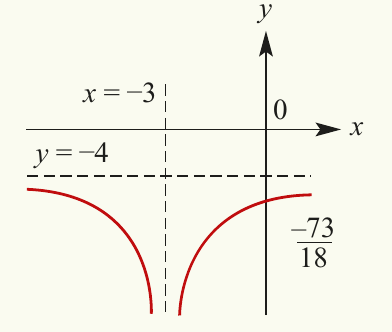
Worked Example: Sketching a Transformed Truncus
Sketch the graph of
Step 1: Identify the parent function
We can think of this as a transformation of the parent function .
Step 2: Describe the transformations
Comparing our function to the general form :
- We have (so the graph is reflected and vertically compressed)
- We have (so the graph is translated 3 units to the left)
- We have (so the graph is translated 4 units down)
The graph of has been translated 3 units to the left and 4 units down.
Step 3: Determine the asymptotes
Using our rules:
- Vertical asymptote: x = -3
- Horizontal asymptote: y = -4
Step 4: Find the y-intercept
To find where the graph crosses the y-axis, we substitute :
The y-intercept is at , which is approximately .
Step 5: Sketch the curve
The graph opens downward (because is negative), is centred at , and has its vertex approaching . The y-intercept gives us one additional point to ensure accuracy.
Remember!
Key Points to Remember:
- The truncus is the graph of , creating a symmetric U-shaped curve with two distinct branches
- The function is undefined at x = 0 and produces only positive values for the basic form
- The basic truncus has asymptotes at (vertical) and (horizontal)
- For transformed graphs in the form , the asymptotes are at and
- The graph is symmetric about its vertical asymptote, making it easier to sketch once you've found key features