Discrete Distributions and Expectation Revision Notes for AQA A-Level Further Maths

Discrete Distributions and Expectation

Introduction to discrete probability distributions

A probability distribution shows how probability is allocated across all possible outcomes of a random experiment. The total probability always equals 1, as one of the outcomes must occur.

When you conduct a random experiment, the outcome is often represented by a discrete random variable - a variable that can only take specific, separate values (not continuous). For example, if you flip a fair coin three times and count the number of heads, this count is a discrete random variable because it can only be 0, 1, 2, or 3.

infoNote

The key feature of discrete random variables is that they take only specific, countable values rather than any value in a continuous range. Common examples include counting outcomes (number of heads, number of successes) or distinct categories (rolling a die).

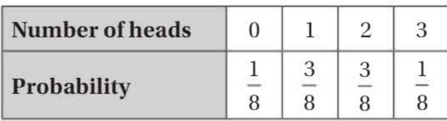
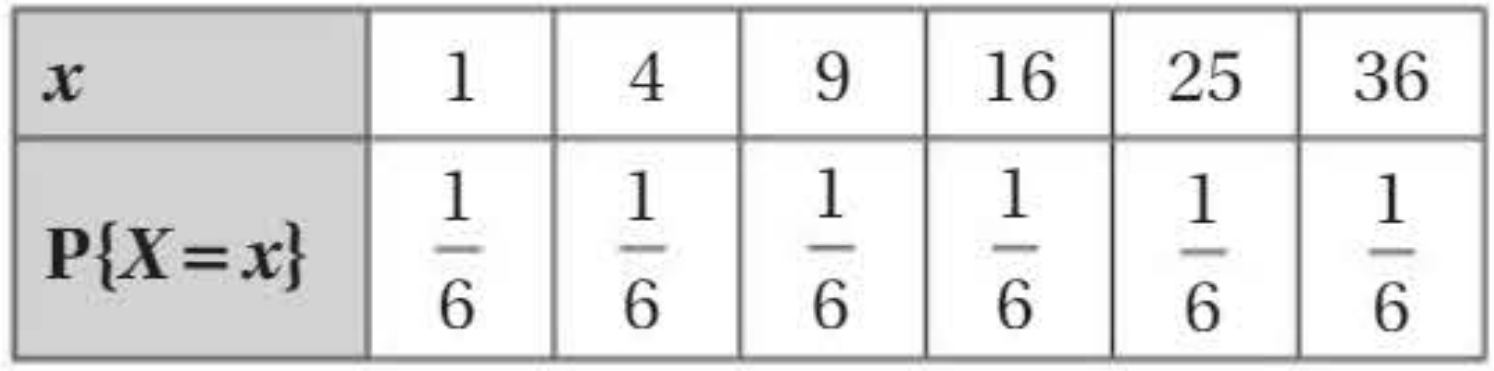
The probability distribution can be presented as a table (as shown above) or as a probability distribution function. For example:

$P(X = x) = \frac{x^2}{30}, \quad x = 1, 2, 3, 4$

This notation means that for each value of $x$ , you substitute it into the formula to find its probability.

Measures of location: median and mode

Just as with data sets, you can calculate measures of location and spread for probability distributions. The two main measures of central tendency for discrete random variables are the median and the mode.

Median

The median of a discrete random variable divides the probability distribution into two equal parts. It's the value where half the probability lies below it and half lies above it.

chatImportant

Definition: The median $M$ of a discrete random variable is the value where:

$P(X \leq M) \geq \frac{1}{2} \text{ and } P(X \geq M) \geq \frac{1}{2}$

This means that at least half the probability is less than or equal to $M$ , and at least half is greater than or equal to $M$ .

Sometimes two distinct values satisfy these inequalities. When this happens, you calculate the median as the arithmetic mean of these two values:

$M = \frac{x_1 + x_2}{2}$

where $x_1$ and $x_2$ are the two values satisfying $P(X \geq x_1) \geq \frac{1}{2}$ and $P(X \leq x_2) \geq \frac{1}{2}$ .

Mode

The mode is much simpler to identify than the median.

infoNote

Definition: For a discrete random variable, the mode is the value with the greatest probability.

In other words, it's the most likely outcome. A random variable may have more than one mode (if multiple values share the highest probability) or may have no mode (if all values have equal probability).

Expected value (expectation)

The expected value of a random variable represents the long-run average outcome you would expect if you repeated the experiment many times. It's also called the mean of the distribution.

To understand this concept, consider throwing a fair die 600 times. The probability of getting a six on any throw is $\frac{1}{6}$ . You would expect to get approximately 100 sixes out of 600 throws. The expected value formalises this idea.

Definition and formula

chatImportant

Definition: The expected value or mean of a discrete random variable $X$ is given by:

$E[X] = \sum_{\forall x} xP(X = x)$

The symbol $\forall$ means "for all", so you sum across all possible values of $x$ .

In words: multiply each possible value by its probability, then add up all these products.

infoNote

The expected value is sometimes denoted by the symbol $\mu$ (Greek letter mu, representing the English letter $m$ for "mean").

How to calculate expected value

To calculate $E[X]$ :

List all possible values the random variable can take
Find the probability of each value
Multiply each value by its probability
Sum all these products

The expected value doesn't have to be a value that the variable can actually take. For example, the expected value of a dice roll is 3.5, even though you can never roll 3.5 on a die!

lightbulbExample

Worked Example: Expected value calculation

Table

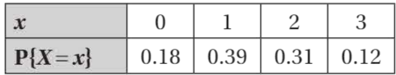
For this distribution:

$E[X] = 0 \times 0.18 + 1 \times 0.39 + 2 \times 0.31 + 3 \times 0.12$
$E[X] = 0 + 0.39 + 0.62 + 0.36 = 1.37$

Expected value of a function

Often you need to find the expected value of a function of a random variable, such as $X^2$ or $3X + 5$ . You can do this by applying the function to each value before multiplying by probabilities.

chatImportant

Formula: The expected value of a function $g(X)$ of a discrete random variable is:

$E[g(X)] = \sum_{\forall x} g(x)P(X = x)$

This means: apply the function $g$ to each possible value $x$ , multiply by the probability $P(X = x)$ , then sum.

lightbulbExample

Worked Example: Expected value of $X$ and $X^2$

Table

Part a: Find $E[X]$

$E[X] = (-1) \times 0.2 + 2 \times 0.3 + 3 \times 0.4 + 5 \times 0.1$ $E[X] = -0.2 + 0.6 + 1.2 + 0.5 = 2.1$

Part b: Find $E[X^2]$

First, calculate $X^2$ for each value:

When $X = -1$ : $X^2 = 1$
When $X = 2$ : $X^2 = 4$
When $X = 3$ : $X^2 = 9$
When $X = 5$ : $X^2 = 25$

Now calculate the expected value:

$E[X^2] = 1 \times 0.2 + 4 \times 0.3 + 9 \times 0.4 + 25 \times 0.1$ $E[X^2] = 0.2 + 1.2 + 3.6 + 2.5 = 7.5$

Notice that $E[X^2] \neq (E[X])^2$ . In this example, $(E[X])^2 = 2.1^2 = 4.41$ , which is different from $E[X^2] = 7.5$ .

Variance and standard deviation

While the expected value tells you about the centre of the distribution, the variance measures how spread out the distribution is around its mean.

Variance definition

infoNote

Definition: The variance of a random variable $X$ measures the expected value of the squared deviations from the mean:

$\text{Var}(X) = E[(X - \mu)^2] = \sum_{\forall x} (x - \mu)^2 P(X = x)$

The variance can also be written as $\sigma^2$ (sigma squared).

Alternative formula for variance

Calculating variance using the definition involves squaring many terms $(x - \mu)^2$ , which can be tedious. There's an alternative formula that's usually much easier to use:

chatImportant

Alternative Formula for Variance:

$\text{Var}(X) = E[X^2] - \mu^2 = E[X^2] - (E[X])^2$

This formula says: the variance equals the mean of the squares minus the square of the mean.

Calculation tip: It's almost always easier to use this alternative formula. Calculate $E[X^2]$ and $E[X]$ separately, then use this formula.

Standard deviation

The standard deviation $\sigma$ is the square root of the variance:

$\sigma = \sqrt{\text{Var}(X)}$

The standard deviation has the same units as the original variable, making it easier to interpret than variance.

lightbulbExample

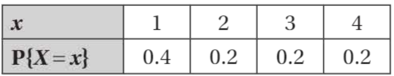
Worked Example: Calculating variance

Consider a random variable $X$ with the probability distribution:

Table

First, calculate $\mu = E[X] = 2.1$ (from earlier)

Next, create a table with values of $x^2$ :

$x$	$-1$	$2$	$3$	$5$
$x^2$	$1$	$4$	$9$	$25$
$P(X=x)$	$0.2$	$0.3$	$0.4$	$0.1$

Calculate $E[X^2]$ :

$E[X^2] = 1 \times 0.2 + 4 \times 0.3 + 9 \times 0.4 + 25 \times 0.1 = 7.5$

Use the alternative formula:

$\text{Var}(X) = E[X^2] - (E[X])^2 = 7.5 - (2.1)^2 = 7.5 - 4.41 = 3.09$

Therefore, the standard deviation is $\sigma = \sqrt{3.09} \approx 1.76$

Variance of a function

Just as with expected values, you can find the variance of a function of $X$ :

$\text{Var}(g(X)) = E[\{g(X)\}^2] - \{E[g(X)]\}^2$

Discrete uniform distribution

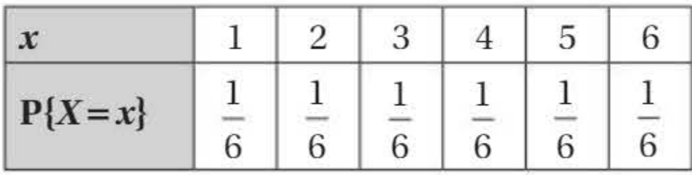
A special type of discrete distribution occurs when all outcomes are equally likely, such as when rolling a fair die.

infoNote

Definition: A discrete uniform random variable $U$ taking values $u = 1, 2, ..., n$ has a probability distribution:

$P(U = u) = \frac{1}{n}, \quad u = 1, 2, ..., n$

Each of the $n$ outcomes has probability $\frac{1}{n}$ .

Formulas for uniform distribution

For a discrete uniform random variable $U$ with values $1, 2, ..., n$ :

chatImportant

Mean: $\mu = E[U] = \frac{n+1}{2}$

Variance: $\sigma^2 = \text{Var}(U) = \frac{n^2-1}{12}$

These formulas save significant calculation time when you recognise a uniform distribution.

lightbulbExample

Worked Example: Fair die

Table

An ordinary fair die gives a uniform distribution with $n = 6$ .

Using the formulas:

$\mu = \frac{6+1}{2} = \frac{7}{2} = 3.5$

$\sigma^2 = \frac{6^2-1}{12} = \frac{36-1}{12} = \frac{35}{12} \approx 2.92$

This is much faster than calculating $E[X]$ and $E[X^2]$ from first principles!

Linear transformations of random variables

When you transform a random variable by multiplying by a constant and/or adding a constant, there are useful rules for how the expectation and variance change.

chatImportant

Key result: If $X$ and $Y$ are two discrete random variables and $Y = aX + b$ , where $a$ and $b$ are constants, then:

$E(Y) = aE(X) + b$ $\text{Var}(Y) = a^2\text{Var}(X)$

You can also write these as $E(aX + b) = aE(X) + b$ and $\text{Var}(aX + b) = a^2\text{Var}(X)$ .

Understanding the rules

Expectation: Both multiplying by $a$ and adding $b$ affect the expected value in a straightforward way. This makes sense - if you double all values ( $a = 2$ ), the average doubles; if you add 5 to all values ( $b = 5$ ), the average increases by 5.

infoNote

Variance: Only the multiplication factor $a$ affects the variance, and it's squared ( $a^2$ ). Adding a constant $b$ doesn't change the spread of the distribution - it just shifts all values by the same amount. The squaring of $a$ occurs because variance involves squared deviations.

Sums of independent random variables

When working with two or more random variables, you often need to find the expected value and variance of their sum.

Expected value of sums

The rule for expected values is beautifully simple:

chatImportant

Key result: For two discrete random variables $X$ and $Y$ , the expected value of their sum is:

$E(X + Y) = E(X) + E(Y)$

This rule works regardless of whether $X$ and $Y$ are independent. The expectations always add.

Variance of sums

The rule for variances has an important restriction:

chatImportant

Key result: For two independent random variables $X$ and $Y$ , the variance of their sum is:

$\text{Var}(X + Y) = \text{Var}(X) + \text{Var}(Y)$

Critical: This rule only works when $X$ and $Y$ are independent. If they're not independent, the variances don't simply add.

lightbulbExample

Worked Example: Football goals

Consider West End FC Under 11s football team. During home games, the number of goals scored has a mean of 3.1 and a standard deviation of 1.2. During away games, the mean is 2.7 and the standard deviation is 1.4.

Let $X$ = goals in home games and $Y$ = goals in away games.

For the total goals $X + Y$ :

$E(X + Y) = E(X) + E(Y) = 3.1 + 2.7 = 5.8$

For variance, we need to assume $X$ and $Y$ are independent:

$\text{Var}(X + Y) = \text{Var}(X) + \text{Var}(Y) = 1.2^2 + 1.4^2 = 1.44 + 1.96 = 3.4$

Therefore, the standard deviation of total goals is:

$\sigma = \sqrt{3.4} \approx 1.84$

Note: The variance result assumes that goals scored in home and away games are independent - that the performance in one doesn't affect the other.

Problem-solving strategy

When solving problems involving expectation and variance:

Find the probability distribution of the random variable (as a table or function)
Use standard formulas to find the mean and variance:
- $E[X] = \sum xP(X=x)$
- $\text{Var}(X) = E[X^2] - (E[X])^2$
Find expectations of functions if needed using $E[g(X)] = \sum g(x)P(X=x)$
Apply transformation rules for linear functions: $E(aX+b) = aE(X)+b$ and $\text{Var}(aX+b) = a^2\text{Var}(X)$
For sums, use $E(X+Y) = E(X) + E(Y)$ and (if independent) $\text{Var}(X+Y) = \text{Var}(X) + \text{Var}(Y)$
State your conclusion clearly

Exam tips

infoNote

Common Pitfalls and Tips:

Always check that probabilities sum to 1 in any distribution - this is a common way to find unknown parameters
The mode is simply the value with the highest probability - don't overcomplicate it
For median, check both inequalities $P(X \leq M) \geq \frac{1}{2}$ and $P(X \geq M) \geq \frac{1}{2}$
Use the computational formula for variance: $\text{Var}(X) = E[X^2] - (E[X])^2$ - it's much faster than the definition
Remember that $E[X^2] \neq (E[X])^2$ - these are different quantities
When applying linear transformations, the constant $b$ doesn't affect variance
The coefficient $a$ is squared in the variance formula: $\text{Var}(aX + b) = a^2\text{Var}(X)$
Expectations always add: $E(X + Y) = E(X) + E(Y)$
Variances only add when variables are independent
For uniform distributions, use the shortcut formulas to save time
Always show your working clearly, especially when using transformation rules or sum rules

bookmarkSummary

Key Points to Remember:

Discrete random variables take only specific, separate values (not continuous)
The mode is the value with the greatest probability - the most likely outcome
The median divides the distribution in half: $P(X \leq M) \geq \frac{1}{2}$ and $P(X \geq M) \geq \frac{1}{2}$
The expected value $E[X] = \sum xP(X=x)$ is the weighted average of all outcomes
Use the computational formula for variance: $\text{Var}(X) = E[X^2] - (E[X])^2$
For linear transformations $Y = aX + b$ : expectations and variances transform as $E(Y) = aE(X) + b$ and $\text{Var}(Y) = a^2\text{Var}(X)$
For sums: expectations always add $E(X+Y) = E(X) + E(Y)$ , but variances only add when variables are independent: $\text{Var}(X+Y) = \text{Var}(X) + \text{Var}(Y)$
For discrete uniform distributions with $n$ values: $\mu = \frac{n+1}{2}$ and $\sigma^2 = \frac{n^2-1}{12}$

Discrete Distributions and Expectation (AQA A-Level Further Maths): Revision Notes