Hypothesis Testing and the t-Test (AQA A-Level Further Maths): Revision Notes
Type II Errors and Power
Understanding errors in hypothesis testing
When conducting hypothesis tests, we can make two types of mistakes: Type I errors and Type II errors. Understanding these errors is crucial for interpreting test results correctly and choosing appropriate significance levels.
In hypothesis testing, we always assume the null hypothesis is true when determining the critical region. The probability of obtaining a result in the critical region should be less than or equal to the test's significance level.
Type I errors
A Type I error occurs when we reject a null hypothesis that is actually true. This is also known as a "false positive" - we conclude there is an effect or difference when there really isn't one.
The probability of making a Type I error is denoted by α (alpha). This probability equals the significance level of the test. For example, if we conduct a test at the 5% significance level, then α = 0.05.
Key formula for Type I error probability:
The important thing to remember is that we can control the probability of a Type I error by choosing our significance level. If we want to be more cautious about false positives, we can use a smaller significance level (like 1% instead of 5%).
Type II errors
A Type II error occurs when we accept (fail to reject) a null hypothesis that is actually false. This is a "false negative" - we miss detecting a real effect or difference.
The probability of making a Type II error is denoted by β (beta). Unlike Type I errors, calculating β is more challenging because it depends on the true value of the population parameter being tested.
Key formula for Type II error probability:
Since we don't usually know the true parameter value in advance, we often calculate β for several possible true values to understand how the test performs. This gives us a picture of when the test might fail to detect a false null hypothesis.
The relationship between Type I and Type II errors
Type I and Type II errors are generally not independent. There's an inverse relationship between them - decreasing one error type typically increases the other.
Understanding the Trade-off:
For instance:
- If we lower the significance level (reduce α), we make it harder to reject H₀, which increases the chance of accepting a false null hypothesis (increases β)
- If we increase the significance level (increase α), we make it easier to reject H₀, reducing β but increasing the risk of rejecting a true null hypothesis
The probability of making a Type I error is much easier to control through the significance level. However, this creates a trade-off that we must consider when designing our test.
The power of a hypothesis test
The power of a hypothesis test tells us how good the test is at detecting when the null hypothesis is false. It's defined as the probability that we correctly reject a false null hypothesis.
Key definition:
The power depends on several factors:
- The true value of the parameter being tested
- The sample size used in the test
- The significance level chosen
Power is rarely a fixed value. Instead, it changes depending on how far the true parameter value is from the value stated in the null hypothesis. The larger the power, the better the test is at avoiding Type II errors.
Generally, we want our test to have high power (close to 1), meaning there's a strong probability of correctly identifying when H₀ is false.
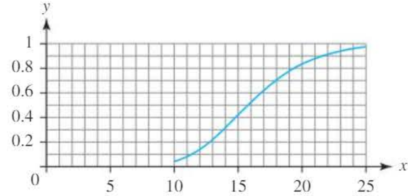
Interpreting the Power Curve:
This graph illustrates how power changes for different true parameter values in a Poisson distribution hypothesis test. Notice that:
- When the true parameter value is close to the null hypothesis value, power is low (near the significance level)
- As the true parameter value moves further from the null hypothesis value, power increases
- Power approaches 1 when the true parameter value is much different from the null hypothesis value
Worked example 1: Poisson distribution
Worked Example: Calculating Type I and Type II Errors for a Poisson Test
Scenario: A Poisson distribution is being tested with null hypothesis λ = 1.9 and alternative hypothesis λ > 1.9. The critical value at the 5% significance level is 5. The true parameter value is λ = 3.1.
Part a: Finding the probability of a Type I error
A Type I error means rejecting a true null hypothesis. The probability equals the probability of getting a result in the critical region when H₀ is true.
Using the Poisson distribution formula:
When λ = 1.9 (the null hypothesis value):
Using the Poisson probabilities with λ = 1.9:
Probability of Type I error = 4.41%
This makes sense because we set our test at the 5% significance level, and the probability should be close to (but not exceed) 5%.
Part b: Finding the probability of a Type II error
A Type II error means accepting a false null hypothesis. We need to find the probability of getting a result outside the critical region when the true parameter value is λ = 3.1.
The critical region is X ≥ 5, so outside this region means X ≤ 4.
When λ = 3.1:
Using the Poisson formula with λ = 3.1:
Probability of Type II error = 79.8%
This is quite high, which tells us that λ = 1.9 and λ = 3.1 are difficult to distinguish with this test. This often happens when the sample situation makes these values hard to tell apart. Using a larger sample size would help reduce this probability.
Worked example 2: Normal distribution
Worked Example: Type II Error and Power for a Normal Distribution Test
Scenario: The mean of a Normal distribution with standard deviation 2.2 is being tested at the 10% level. The null hypothesis is μ = -0.8 and the alternative hypothesis is μ ≠ -0.8. The true mean is μ = -3.2.
Part a: Finding the probability of a Type II error
For this two-tailed test at the 10% level, we need to find the critical region first. Each tail contains 5% of the distribution.
Using the Normal distribution with mean -0.8 and standard deviation 2.2:
- Lower critical value: X < -4.42
- Upper critical value: X > 2.82
When the true mean is μ = -3.2, we need to find the probability of obtaining a value outside these critical regions.
With μ = -3.2 and σ = 2.2:
This can be written as:
Using the Normal distribution:
Probability of Type II error = 70.7%
Part b: Calculating the power
The power is simply:
Power = 0.293 or 29.3%
This relatively low power indicates that when the true mean is -3.2, there's only about a 29% chance of correctly rejecting the false null hypothesis. The test isn't very effective at distinguishing between μ = -0.8 and μ = -3.2 with the current setup.
Worked example 3: Effect of significance level on Type II errors
Worked Example: How Significance Level Affects Type II Error Probability
Scenario: A Normal distribution with standard deviation 4 is being tested with hypotheses H₀: μ = 7.7 and H₁: μ < 7.7. The true mean is 2.5. We'll examine how the probability of a Type II error changes at different significance levels.
At 10% significance level
For a one-tailed test at 10%: Critical value = 2.57
The Type II error probability is:
Type II error = 40.3%
At 5% significance level
For a one-tailed test at 5%: Critical value = 1.12
The Type II error probability is:
Type II error = 63.5%
At 1% significance level
For a one-tailed test at 1%: Critical value = -1.61
The Type II error probability is:
Type II error = 84.8%
Important observation
Notice that relatively small changes to the significance level have brought large changes to the probability of making a Type II error. As we make our test more conservative (lower significance level), we substantially increase the risk of missing a false null hypothesis.
This demonstrates the crucial trade-off in hypothesis testing: being more cautious about Type I errors makes us more vulnerable to Type II errors.
Practical considerations for choosing significance levels
When designing a hypothesis test, consider which type of error has more serious consequences in your specific situation.
Strategy 1: Prioritising Type I or Type II errors
You should decide whether it's more important to reduce the probability of a Type I error or a Type II error. Different situations call for different priorities.
Example - Medical testing:
When testing a new medical treatment for a rare illness with the null hypothesis "the person does not have the illness":
- Type II error: Accepting H₀ when it's false means not diagnosing someone who genuinely has the illness. This could be very serious as they won't receive treatment.
- Type I error: Rejecting H₀ when it's true means diagnosing someone who doesn't have the illness. While concerning, this can often be caught with a repeat test.
In this context, we want to minimise the Type II error, even if it means accepting a higher Type I error rate. Missing a genuine illness is worse than a false positive that can be checked again.
Strategy 2: Sample size considerations
The sample size should be large enough so that if the true value is very different from the null hypothesis, the result is likely to fall inside the critical region.
If the true parameter value and the null hypothesis value are similar, they become difficult to distinguish. A larger sample size helps to:
- Reduce the probability of Type II errors
- Increase the power of the test
- Make it easier to detect even small differences from H₀
When the true parameter value is much different from the null hypothesis value, even a moderate sample size will usually give the test good power (approaching 1).
Understanding power curves
Power curves show how the power of a test changes as the true parameter value varies. These graphs help us understand when our test is effective and when it might struggle.
Key features of power curves:
- Power is low when the true parameter value is close to the null hypothesis value
- Power increases as the true value moves further from H₀
- Power approaches 1 when the true value is very different from H₀
- The power is never technically defined when the null hypothesis is actually the true value (since power measures rejection of a false H₀)
For example, if we're testing H₀: λ = 10 versus H₁: λ > 10 for a Poisson distribution, the power exceeds 0.5 when the true value is around 15.7. This means there's a better-than-even chance of correctly rejecting the false null hypothesis when λ ≥ 15.7.
Key Points to Remember:
- Type I error (α): Rejecting a true null hypothesis - controlled by the significance level
- Type II error (β): Accepting a false null hypothesis - depends on the true parameter value
- Power = 1 - β: The probability of correctly rejecting a false null hypothesis - we want this to be high
- Trade-off: Decreasing Type I errors typically increases Type II errors, and vice versa
- Context matters: Choose your significance level based on which error type has more serious consequences in your specific situation