The t-Test (AQA A-Level Further Maths): Revision Notes
The t-Test
Introduction to the t-test
When conducting hypothesis tests about the mean of a Normal distribution, the method depends on whether the population variance is known. If the population variance is known, you can use a standard Normal distribution test (z-test). However, when the population variance is unknown, which is often the case in real-world situations, you must use a different approach called the t-test.
The t-test uses the sample variance as an estimate for the unknown population variance. This estimation introduces additional uncertainty, particularly when working with small sample sizes. The t-test accounts for this extra uncertainty by using a different probability distribution called the t-distribution.
The key distinction between using a z-test and a t-test lies in whether you know the population variance. In most practical situations, you won't know the true population variance, making the t-test the appropriate choice for small samples.
Understanding the sample mean distribution
Consider a situation where you believe a process follows a Normal distribution with an expected mean of 12.0. You collect a sample of 10 observations:
| 11.9 | 8.37 | 14.8 | 14.6 | 11.2 |
| 11.1 | 14.9 | 12.2 | 10.7 | 15.7 |
The sample mean of these values is . This value is relatively close to the hypothesised population mean of 12.0, but it could also be far from it depending on the variability in the data. To make a proper decision, you need to understand the probability distribution of the sample mean.
The sample mean is itself a random variable with its own probability distribution. An important statistical principle states that the mean of the sample mean distribution (also called the expected value of ) equals the population mean . In other words, on average, the sample mean provides an unbiased estimate of the population mean. However, any individual sample mean may differ from the population mean due to random variation.
The t-distribution
Just as there is a standard Normal distribution that other Normal distributions can be related to, there are standard t-distributions that describe the distribution of sample means for different sample sizes.
When you know the population variance , the test statistic:
follows a standard Normal distribution with mean 0 and variance 1.
However, when the population variance is unknown, you must estimate it using the sample variance. This estimate becomes less reliable as the sample size decreases. The sample variance for a sample of size is calculated as:
Note the divisor is rather than . This correction makes the sample variance an unbiased estimator of the population variance. This is crucial for the t-test to work correctly.
For the sample data shown earlier with :
The t-distribution is similar in shape to the Normal distribution (bell-shaped and symmetric) but has heavier tails, meaning it assigns greater probability to extreme values. This reflects the additional uncertainty from estimating the population variance. The exact shape of the t-distribution depends on the degrees of freedom, which for a single-sample t-test equals .
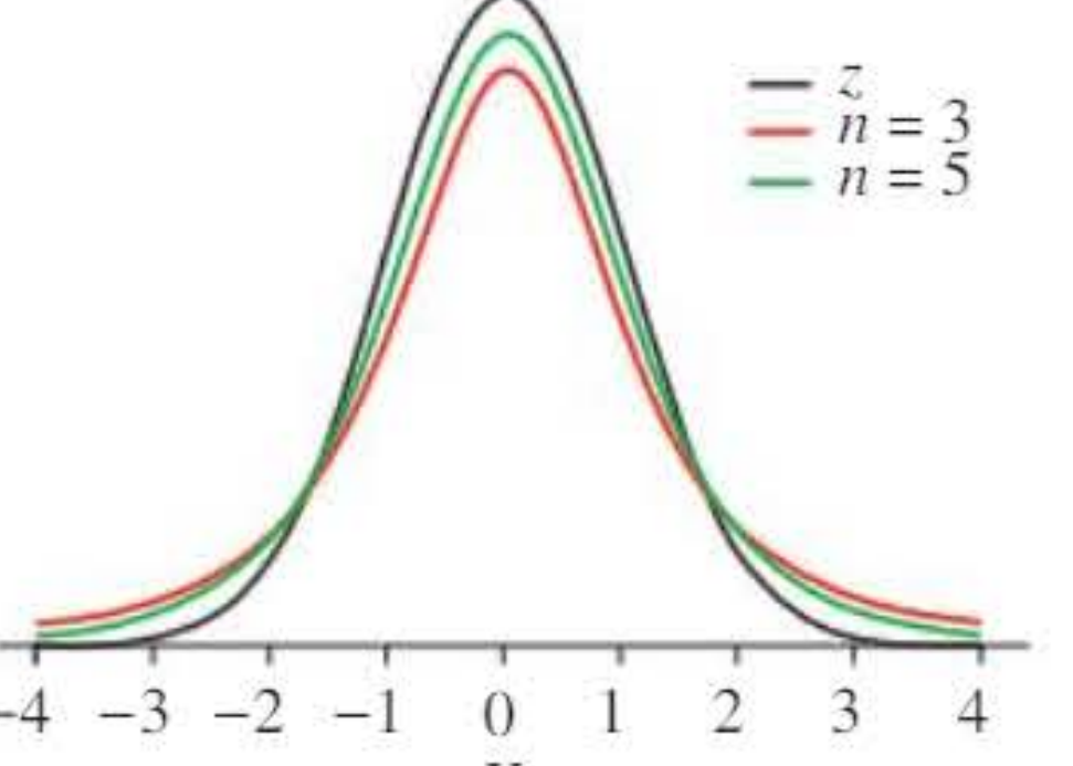
As the sample size increases, the t-distribution becomes increasingly similar to the standard Normal distribution. When the degrees of freedom approach infinity (very large samples), the t-distribution becomes identical to the standard Normal distribution.
The t-test statistic
The t-test statistic is calculated using the formula:
where:
- is the sample mean
- is the hypothesised population mean (from the null hypothesis)
- is the sample standard deviation (the square root of the sample variance)
- is the sample size
The test statistic follows a t-distribution with degrees of freedom.
Degrees of freedom
The degrees of freedom represent the number of independent pieces of information available to estimate the population variance. For a single-sample t-test, the degrees of freedom equal:
We subtract 1 because we use the sample mean to calculate the sample variance, which constrains one degree of freedom. Always remember: degrees of freedom = , not !
Conducting a hypothesis test using the t-test
The procedure for conducting a t-test follows the standard hypothesis testing framework:
Step 1: State the hypotheses
- Null hypothesis : (population mean equals hypothesised value)
- Alternative hypothesis : This depends on the context (could be , , or )
Step 2: Choose a significance level (e.g., 5%, 10%, 1%)
Step 3: Calculate the test statistic using
Step 4: Find the degrees of freedom: df =
Step 5: Determine the p-value or critical region using the t-distribution tables or calculator
Step 6: Make a decision by comparing the p-value to the significance level, or by checking if the test statistic falls in the critical region
Step 7: State your conclusion in context
Worked Example 1: Calculating the t-test statistic
Using the sample data from earlier (mean = 12.547, sample variance = 5.56, ), test whether the population mean is 12.0.
The test statistic is:
Using the t-distribution with degrees of freedom, the probability of obtaining a sample mean this large or larger is 24.1%.
Conclusion: Since no significance level was stated, but 24.1% is quite large (much greater than typical significance levels like 5% or 10%), it is reasonable to conclude that the sample could have come from a Normal distribution with mean 12.0. There is insufficient evidence to reject the null hypothesis.
Worked Example 2: Complete hypothesis test
A population following a Normal distribution with unknown variance is being tested at the 10% significance level. The hypotheses are:
A sample of size 8 is taken, which has a sample mean of 2.39 and a sample variance of 1.12.
a) Calculate the t-test statistic
b) State the number of degrees of freedom
Degrees of freedom =
c) Calculate the p-value of the statistic
Using a calculator or t-distribution tables with 7 degrees of freedom:
Since this is a two-tailed test (the alternative hypothesis is ), we need to consider both tails. However, the calculator gives us the cumulative probability for one tail.
d) Determine the conclusion of the test
This is a two-tailed test, so we compare the one-tail probability to half the significance level: (where 5% is half of 10%).
Alternatively, we can double the one-tail probability: .
Conclusion: Since the p-value is less than the significance level, there is significant evidence to reject the null hypothesis. We conclude that the sample is not likely to have come from a population Normal distribution with mean 3.2.
Confidence intervals using the t-distribution
The t-distribution can also be used to construct confidence intervals for the population mean when the population variance is unknown and the sample size is small.
For a sample of size taken from a Normal distribution , the -confidence interval is:
where:
- is the critical value from the t-distribution with degrees of freedom
- is the sample mean
- is the sample standard deviation (or )
For a -confidence interval, you need to find using your calculator's inverse t-distribution function.
Worked Example 3: Constructing a confidence interval
A sample of size 16 is taken with a mean of 13.6 and a standard deviation of 20.4. Generate a 95% confidence interval for the population mean.
For and with degrees of freedom:
(Note: We use 0.975 because )
The confidence interval is:
This simplifies to:
Interpretation: We are 95% confident that the true population mean lies between 2.74 and 24.46.
When to use the t-test vs Normal test
Understanding when to use each test is crucial for exams:
Use the t-test when:
- The population variance is unknown
- The sample comes from a Normal population
- The sample size is small (typically )
Use the Normal distribution test (z-test) when:
- The population variance is known
- OR the sample size is large (typically )
A good rule of thumb: If the sample size is larger than 30, the t-distribution is numerically close enough to the standard Normal distribution that you can use the Normal distribution instead. This is because as the degrees of freedom increase, the t-distribution converges to the standard Normal distribution.
Conditions for validity
For a hypothesis test using the t-distribution to give valid results, two conditions must be met:
Validity Conditions for the t-test:
- The population must be Normally distributed (or approximately Normal)
- The sample must be taken randomly (to avoid bias)
If either condition is violated, the t-test results may not be reliable.
Worked Example 4: Identifying invalid test conditions
A student wants to test whether the average number of devices that can connect to the internet per UK household is five or greater. They ask seventeen friends to record their values and decide to use a t-test due to the small sample size.
Why will this test not give a valid result?
Reason 1: Non-random sample The sample is not random. The student is asking their friends, which introduces bias. Friends of the student are likely to have similar characteristics (e.g., similar age, socioeconomic status, tech-savviness), making the sample unrepresentative of all UK households.
Reason 2: Violation of Normality assumption The values are unlikely to be approximately Normally distributed. The number of devices is discrete and likely skewed, so the assumption of Normality is violated, making the t-test unsuitable.
Key formulas summary
Sample variance:
t-test statistic:
Degrees of freedom:
Confidence interval:
Exam tips and common traps
Tip 1: Always check whether the variance is known or unknown. If it's unknown, use the t-test; if it's known, use the Normal distribution.
Tip 2: Don't forget to subtract 1 when calculating degrees of freedom. It's n - 1, not .
Tip 3: For two-tailed tests, remember to consider both tails of the distribution when finding p-values or critical regions.
Tip 4: When stating conclusions, always write them in context. Don't just say "reject " – explain what this means for the original problem.
Tip 5: Check validity conditions before using the t-test. If the sample isn't random or the population isn't Normal, the test results may not be valid.
Common trap: Students often confuse the sample variance formula for the t-test ( with divisor ) with the population variance or the biased sample variance (divisor ). Always use for the t-test.
Common trap: Forgetting to take the square root when calculating the denominator of the t-statistic. The formula has , not .
Common trap: Using the wrong distribution. If or if the variance is known, you should typically use the Normal distribution, not the t-distribution.
Remember!
Key Points to Remember:
-
The t-test is used when testing a population mean from a Normal distribution with unknown variance, particularly when the sample size is small ().
-
The t-test statistic is and follows a t-distribution with degrees of freedom.
-
The t-distribution has heavier tails than the Normal distribution, reflecting greater uncertainty when estimating the population variance from sample data.
-
As sample size increases, the t-distribution converges to the standard Normal distribution. For , you can typically use the Normal distribution instead.
-
For the t-test to be valid, the population must be Normally distributed and the sample must be random. Always check these conditions before applying the test.