Aggregate Demand (Edexcel A-Level Economics A): Revision Notes
Aggregate Demand
Aggregate demand represents the total level of spending on goods and services within an economy over a specific time period. Understanding how aggregate demand functions is essential for analysing macroeconomic performance, as it helps explain how different sectors of the economy interact and how changes in spending patterns affect overall economic activity.
When examining aggregate demand, economists break it down into distinct components, each representing spending by different economic agents. By understanding what determines the level of each component, we can better analyse how the economy operates and predict how it might respond to various economic changes or policy interventions.
The components of aggregate demand
Aggregate demand refers to the total amount of spending on goods and services produced within an economy during a given period. This spending comes from four main sources: households, firms, government, and the international sector. Each of these contributes to the overall level of demand in different ways.
The relationship between these components can be expressed mathematically as:
Where:
- AD represents aggregate demand
- C represents consumption (household spending)
- I represents investment (spending by firms on capital goods)
- G represents government spending
- X represents exports (foreign spending on domestic goods)
- M represents imports (domestic spending on foreign goods)
We use net exports because imports represent spending that leaves the domestic economy and therefore needs to be subtracted from total spending. When imports exceed exports, this creates a negative contribution to aggregate demand, as it represents money flowing out of the domestic economy.
UK aggregate demand breakdown
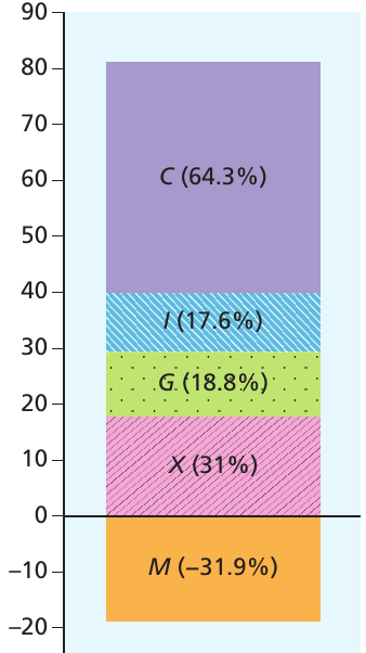
To illustrate the relative importance of each component, we can examine real-world data. In the UK during 2019, the expenditure-side breakdown showed the following pattern:
| Component | Percentage of GDP |
|---|---|
| Consumption (C) | 64.3% |
| Investment (I) | 17.8% |
| Government expenditure (G) | 18.8% |
| Exports (X) | 31% |
| Imports (M) | -31.9% |
This data reveals several important points. Consumption forms by far the largest component of aggregate demand, accounting for nearly two-thirds of total GDP. However, the government expenditure figure of 18.8% somewhat understates the overall significance of public sector spending, as it excludes public investment in infrastructure and services, which is included within the investment figure. When combined, public and private sector investment made up 17.6% of total GDP, highlighting the importance of capital formation in the economy.
Notice that imports exceeded exports, resulting in a negative trade balance. This means the UK spent more on goods and services from abroad than it earned from selling its own products overseas. This negative net trade position reduces the overall level of aggregate demand in the economy.
Consumption
Consumption represents the single largest component of aggregate demand in most developed economies. Consumption refers to total planned household spending on goods and services. Understanding what drives consumption is therefore crucial for understanding overall economic performance.
Keynesian consumption theory
The influential economist John Maynard Keynes, whose major work The General Theory of Employment, Interest and Money was published in 1936, proposed that the most important factor determining consumption is disposable income. Disposable income is the income that households actually have available to spend on consumption or to save, after accounting for direct taxes paid and transfer payments received.

Transfer payments refer to situations where transfers of goods or services occur between individuals or groups without any production taking place. A common example is social security benefits provided by the government, such as Universal Credit or the State Pension. These payments transfer purchasing power from taxpayers to benefit recipients without requiring any work or production in return.
Keynes's key insight was that as real incomes increase, households will tend to spend more on consumption. However, they will not spend all of any income increase - instead, they will save some portion of it. This behaviour can be quantified using two important concepts: the average propensity to consume and the marginal propensity to consume.
Propensities to consume and save
The average propensity to consume (APC) measures the proportion of total income that households devote to consumption. It is calculated by dividing total consumption by total income. For example, if household consumption is \£80 and disposable income is \£100, then , meaning households spend 80% of their income on consumption.
The marginal propensity to consume (MPC) measures the proportion of any additional income that households would devote to consumption. This is calculated by dividing the change in consumption by the change in income.
Worked Example: Calculating the Marginal Propensity to Consume
If disposable income increases from \£100 to \£110 and consumption rises from \£80 to \£87, we can calculate the MPC as follows:
This means that for every additional \£100 of income, \£70 would be spent on consumption and \£30 would be saved.
Similarly, the marginal propensity to save (MPS) measures the proportion of any increase in disposable income that households would devote to saving. Since any income must be either consumed or saved, must always equal 1.
Quick Calculation Tip
If you know the MPC, you can immediately calculate the MPS by subtracting the MPC from 1.
For example, if , then:
This means that for every additional \£100 of income received by households, \£70 would be consumer expenditure and the remaining \£30 would be saved.
The consumption function
The relationship between consumption and income is known as the consumption function. This relationship is shown graphically below, with consumption on the vertical axis and real income on the horizontal axis.
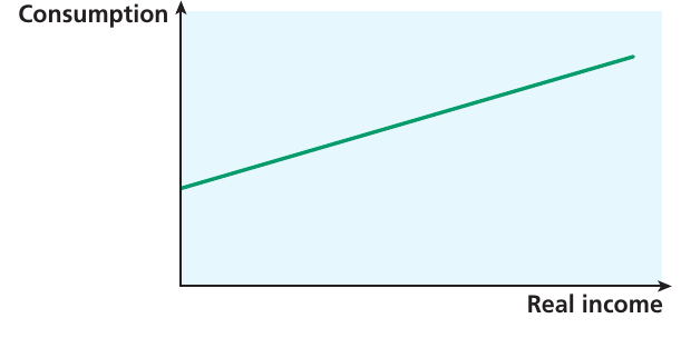
The consumption function has a positive slope, reflecting the fact that as income increases, consumption also increases. The line intercepts the vertical axis above the origin, indicating that there is some level of autonomous consumption - spending that occurs even when income is zero, which would be financed by borrowing or running down savings. The slope of the line represents the marginal propensity to consume.
When examining actual data for the UK, the theoretical relationship holds remarkably well. The scatter plot below shows real household consumption and disposable income from 1997 to 2021, with a fitted trend line demonstrating the strong positive relationship.
Other influences on consumption
While income represents the most important determinant of consumption, several other factors can also affect household spending decisions. These additional influences help explain why consumption patterns may vary even when income levels remain constant.
Wealth effects occur when changes in household wealth lead to changes in consumer spending. Wealth refers to the accumulation of assets over time, which differs from income (the flow of money received per period). If households experience an increase in the value of their assets - particularly house prices or stock market investments - they may feel more financially secure and increase their consumption, even if their current income hasn't changed. This is sometimes called the "wealth effect" or "housing wealth effect". Conversely, falling house prices or stock market crashes can reduce consumption as households feel less wealthy and more cautious about spending.
Interest rates can influence consumption through multiple channels. When interest rates rise, the cost of borrowing increases, which may discourage consumption financed through credit cards, personal loans, or overdrafts. Higher interest rates also make saving more attractive, as the return on savings increases. Additionally, interest rate changes can affect asset prices and therefore trigger wealth effects. Finally, if households expect inflation to increase, they may adjust their consumption patterns accordingly.
Interest rate effects may not be instantaneous - consumption patterns can take time to adjust to changes in economic conditions. The full impact of interest rate changes on household spending decisions may take several months or even quarters to materialise fully.
Consumer confidence plays a significant role in spending decisions. The overall health of the economy and the confidence of individual consumers affect their willingness to spend. Households may increase consumption during periods of economic optimism, when job security seems strong and future income prospects look positive. Conversely, during recessions or periods of uncertainty, even households with stable incomes may reduce spending and increase precautionary savings. Confidence can be influenced by trends in house prices, stock markets, employment prospects, or broader global economic conditions.
Analysing Consumption in Exams
When analysing consumption, disposable income is the primary factor to consider. However, a comprehensive analysis should also acknowledge the secondary influences of wealth, interest rates, and consumer confidence. These factors help explain short-term variations in consumption that income alone cannot account for.
A strong answer will explain the income-consumption relationship first, then discuss how other factors might modify this basic relationship in specific economic circumstances.
Investment
The second major component of aggregate demand is spending by firms on capital goods. Investment refers to expenditure undertaken by firms on physical capital that will be used in the production process. This is an important distinction - in economics, investment specifically means purchasing productive capital, not financial investments like buying shares or putting money in a bank account.

Investment increases the economy's productive capacity by expanding the stock of capital available for production. The capital stock includes plant and machinery, vehicles and transport equipment, and buildings including new dwellings that provide housing services over extended periods.
Types of investment
Gross investment represents the total investment undertaken by firms, comprising two distinct components. The first component is replacement investment, which occurs when firms replace capital that has worn out or become obsolete. This relates to depreciation (or capital consumption), which is the fall in the value of capital goods due to wear and tear over time. The second component is investment to expand productive capacity - adding to the capital stock rather than merely maintaining it.
Net investment is calculated by subtracting depreciation from gross investment:
It represents investment that genuinely adds to the economy's capital stock, net of the replacement of existing capital.
Understanding Net Investment
- If gross investment exceeds depreciation, net investment is positive and the economy's productive capacity is expanding
- If gross investment merely matches depreciation, the capital stock remains constant
- If gross investment falls below depreciation, net investment is negative and productive capacity is actually shrinking
Determinants of investment
Several key factors influence firms' decisions about how much to invest. Understanding these determinants helps explain fluctuations in investment spending and, consequently, in aggregate demand.
Expectations about future demand
The overall state of the economy significantly influences investment decisions. When the economy experiences rapid growth and this growth is expected to continue, firms become optimistic about future demand for their products. This optimism encourages them to invest in new capacity to exploit anticipated profit opportunities. Conversely, during recessions or periods of economic uncertainty, expectations about future demand become more pessimistic, causing firms to hesitate before committing to new investment projects.
Keynes emphasised the role of business psychology in investment decisions, referring to the "animal spirits" of firms - their instinctive optimism or pessimism about economic prospects. During severe recessions, falling confidence can create a self-reinforcing cycle: as investment expenditure falls, the recession deepens, further dampening confidence and delaying recovery.
Expectations about future demand are shaped not only by domestic economic conditions but also by international competitiveness, particularly for firms involved in exporting. Strong overseas demand can encourage investment even when domestic conditions are weak. However, global recessions, such as the financial crisis of the late 2000s and the COVID-19 pandemic, can severely damage confidence across many countries simultaneously, causing widespread reductions in investment.
Government incentives
Government policy can significantly influence the level and pattern of investment. Governments have an interest in encouraging investment because of its beneficial effects on expanding productive capacity and promoting economic growth. Various policy tools can be used to stimulate investment.
Tax concessions represent one approach, potentially reducing the tax burden on firms that undertake investment. Governments may also use regulation to influence where investment occurs - for example, by directing funding toward regions that have struggled to attract private investment. The UK government's "levelling-up" agenda exemplifies this approach, incorporating investment in transport infrastructure, education, the NHS, police forces, and broadband coverage in areas with lower economic development.
Some economists argue that high inflation damages the economy by creating uncertainty about the future, which undermines business confidence and discourages investment. From this perspective, maintaining price stability becomes an important precondition for sustained investment growth.
These various factors combine to determine the overall climate for investment. While firms ultimately decide whether to invest based on expected profitability, the cost and availability of finance, along with government policies, create the environment in which those decisions are made.
Investment and the interest rate
The cost of financing investment projects represents another crucial consideration. The interest rate reflects the cost of borrowing, so when firms need to borrow to fund investment, higher interest rates may discourage investment spending. However, it's important to recognise that not all investment requires borrowing - firms can also use retained profits from previous periods to finance new projects.
Even when using internal funds, the interest rate remains relevant because it represents an opportunity cost. When firms hold cash that could be used for investment, they face a choice: invest in physical capital or purchase financial assets that earn interest. The rate of interest therefore reflects the return foregone by choosing investment over financial assets.
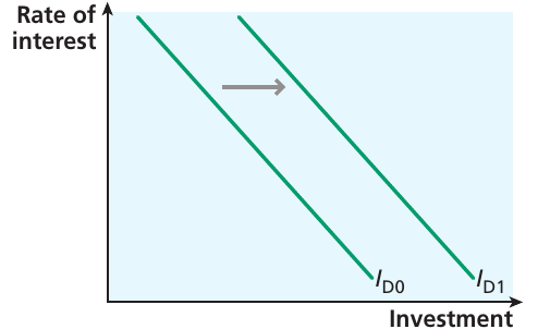
The investment demand function shows an inverse relationship between the interest rate and the level of investment. When interest rates are high, investment is relatively low. The function slopes downward, indicating that lower interest rates encourage greater investment. An improvement in business confidence would shift the entire investment demand function outward (from to in the diagram), meaning that more investment would occur at any given interest rate.
Firms' willingness to borrow depends not only on interest rates but also on the availability of credit. Financial institutions must be willing to lend and must have funds available. Following the financial crisis, many commercial banks became reluctant to lend, having become more risk-averse. The availability of credit also depends on household saving behaviour - bank deposits from savers provide funds that banks can lend to businesses. During and after the crisis, very low interest rates meant poor returns on savings, which reduced the funds available for lending to investors.
Case Study: Investment and the Financial Crisis
Investment in capital goods represents expenditure on produced resources that will be used in future production. This expenditure contributes to economic growth by providing the capital resources needed to increase productive capacity.
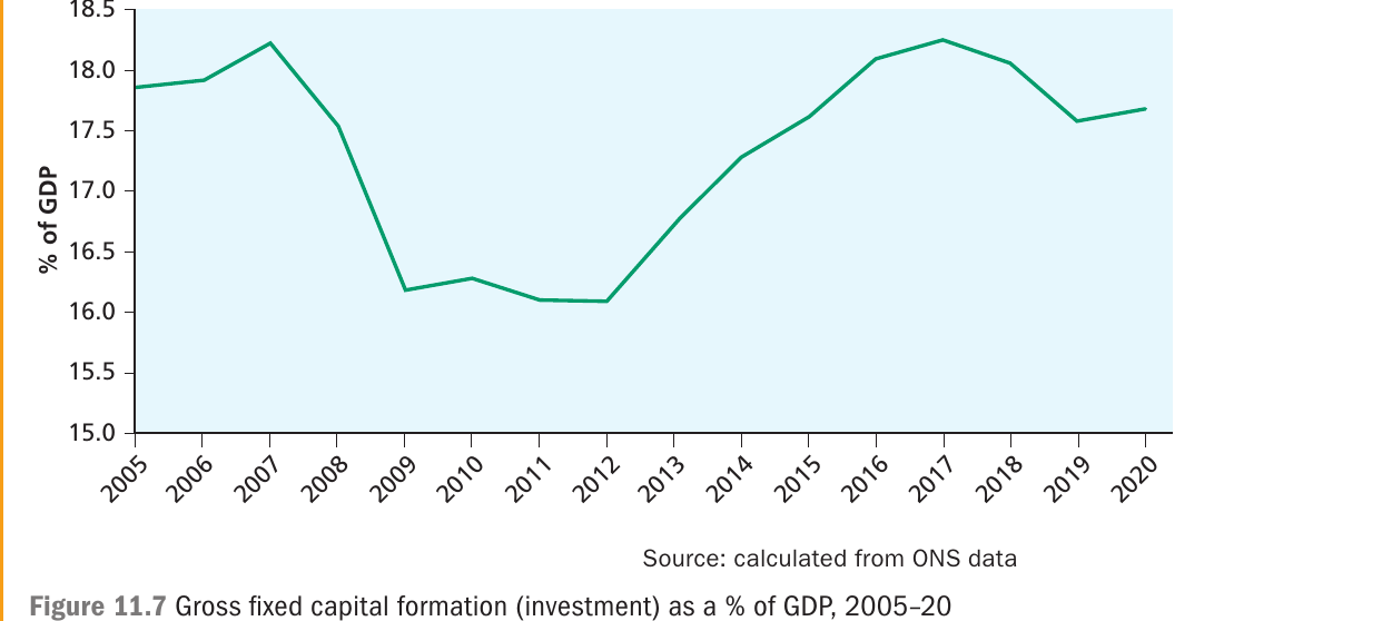
The chart below shows investment in the UK as a percentage of GDP from 2005 to 2020, measured using gross fixed capital formation (the ONS term for investment in national accounts).
Key Observations:
The data clearly shows the impact of the global financial crisis of the late 2000s. Investment fell sharply as a percentage of GDP during the crisis period and remained depressed for several years afterward. Recovery was slow, with investment only returning to pre-crisis levels by around 2017, before declining slightly again by 2020.
Analysis:
The amount of investment undertaken depends on multiple factors. Firms need to generate profits to remain viable, and investment represents one way of improving profit prospects in competitive markets. Investment spending now brings benefits in the future, although costs are incurred in the present. For example, investment in new factory capacity requires immediate expenditure, but the benefits only materialise gradually as production increases over time.
Firms' expectations about future demand heavily influence their investment decisions. During the financial crisis and its aftermath, pessimistic expectations about economic recovery discouraged investment, contributing to the prolonged period of weak capital formation. The slow recovery in investment levels demonstrates how damaged confidence can persistently suppress this crucial component of aggregate demand.
Government expenditure
By and large, government spending decisions follow different criteria from those governing private sector expenditure. The government's role in the economy differs fundamentally from that of households and firms.
When examining macroeconomic equilibrium, government expenditure can often be treated as largely autonomous - that is, independent of the variables being analysed in aggregate demand and supply models. The government makes spending decisions based on policy objectives rather than in direct response to changes in national income or price levels.
However, some elements of government expenditure do vary automatically with economic conditions. Economies experience regular fluctuations known as the business cycle or trade cycle. During recessions, unemployment rises, causing more workers to claim social security benefits, which increases government expenditure. Simultaneously, falling incomes reduce income tax receipts, decreasing government revenue. The reverse occurs during recovery periods: as employment rises, benefit payments fall and tax revenues increase.
Automatic Stabilisers
This pattern creates automatic changes in net government spending that vary countercyclically with economic activity. These are known as automatic stabilisers because they naturally moderate economic fluctuations without requiring any deliberate policy changes.
During recessions:
- Government spending on benefits increases automatically
- Tax revenues decrease automatically
- This provides support to aggregate demand without policy intervention
During booms:
- Government spending on benefits decreases automatically
- Tax revenues increase automatically
- This helps prevent the economy from overheating
Beyond automatic stabilisers, governments can deliberately manipulate spending levels through discretionary fiscal policy. By adjusting taxation and expenditure decisions, governments can influence the trajectory of aggregate demand. This active use of fiscal policy provides a tool for managing economic performance, which we will explore in detail in later chapters on macroeconomic policy.
The UK government adopted an unusually active fiscal stance during the COVID-19 pandemic. Recognising the threat to both public health and economic stability, the government implemented unprecedented interventions, including extensive business support schemes, furlough payments to maintain employment, and increased health service funding. These measures involved government spending on a scale never previously experienced, with significant implications for the national debt.
Synoptic Link: Fiscal Policy
The role of fiscal policy as an economic management tool is examined thoroughly in Chapter 32, which discusses automatic stabilisers, discretionary fiscal changes, and the significance of national debt.
Net trade (X − M)
Finally, we need to consider the factors influencing the level of exports and imports. For economies engaged in international trade, the spending patterns of the rest of the world matter significantly.
Most goods traded internationally are normal goods, meaning demand increases with income. Therefore, as real incomes rise domestically over time, there will be increased demand for imported goods (positive income elasticity of demand). The spending by UK residents on goods and services from abroad represents a withdrawal from the circular flow of income in the UK economy. Conversely, the demand for UK exports depends on income changes in the countries that are the UK's trading partners. When economic growth accelerates abroad, this will impact aggregate demand in the UK through increased export orders. The global recession that emerged during the late 2000s had a significant dampening effect on world trade, affecting economies worldwide.
The exchange rate between sterling and other currencies significantly affects both exports and imports. The exchange rate determines the relative prices of UK goods compared with those produced overseas. When the sterling exchange rate increases (appreciation), UK exports become less competitive in foreign markets because they become more expensive for overseas buyers. Simultaneously, imports into the UK become more competitive because foreign goods become cheaper for UK consumers. An increase in the exchange rate therefore tends to reduce net exports, while a fall in the exchange rate (depreciation) makes UK exports more competitive and imports less competitive, potentially increasing net exports.
Protectionist Policies and International Trade
International trade volumes can also be affected by protectionist policies that countries introduce to shield their domestic industries. Historically, many countries imposed tariffs (taxes on imports), and the import duties collected represented significant government revenue. After the Second World War, tariff rates fell substantially as countries recognised the benefits of specialisation and international trade.
However, tariffs have not disappeared entirely, and countries have also developed non-tariff barriers that restrict trade. These might include regulations imposing strict quality controls on imported goods or other measures designed to limit international competition. In 2018, concerns about trade wars emerged as President Trump raised tariffs on imports from China, which was later extended to EU countries, prompting retaliatory action.
The relative prices of goods produced domestically versus abroad also influence the demand for exports and imports. When UK inflation runs high relative to other countries, this tends to make UK exports less competitive while making imports more attractive. Changes in exchange rates can partially offset changes in relative prices between countries. For example, if UK prices rise faster than prices abroad, this would normally reduce competitiveness, but if the exchange rate also falls, the competitive disadvantage may be neutralised.
Understanding Autonomous Government Expenditure
Understanding that government expenditure can be treated as autonomous is important for analysing macroeconomic models. Autonomous means independent of the model's variables, so government spending doesn't automatically respond to changes in national income or price levels. However, through deliberate policy choices, governments can adjust spending to influence economic outcomes.
The aggregate demand curve
Having examined the individual components of aggregate demand, we can now consider the relationship between aggregate demand and the overall price level. The aggregate demand (AD) curve shows the relationship between the level of aggregate demand and the overall price level. More formally, it represents planned expenditure at any given possible overall price level.
This is fundamentally different from the microeconomic demand curves studied earlier. Microeconomic demand curves show the relationship between the quantity demanded of an individual product and its own price. The aggregate demand curve, by contrast, shows the relationship between the total demand for all goods and services in the economy and the average price level across all products. Aggregate demand comprises all the components we have discussed - consumption, investment, government spending, and net exports - and the price level represents an average of all prices of goods and services throughout the economy.
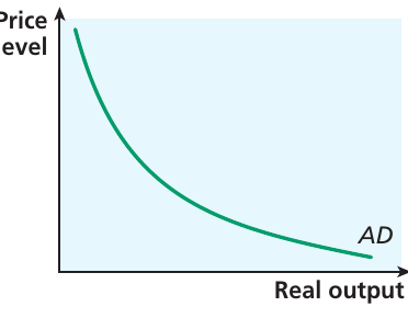
Why the AD curve slopes downward
The aggregate demand curve slopes downward, indicating an inverse relationship between the price level and the quantity of real output demanded. Several mechanisms explain this negative slope.
The real balance effect
When the overall price level is relatively low, the purchasing power of income is relatively high. Low prices mean that any given amount of money income can purchase more goods and services, representing relatively high real income. Additionally, when prices are low, this increases the real value of households' wealth. Consider a household that owns a financial asset such as a bond with a fixed money value of \£100. The relative (real) value of that asset is higher when the overall price level is low compared to when prices are high.
The Real Balance Effect
These considerations suggest that, ceteris paribus (other things being equal), a low overall price level corresponds to relatively high consumption. Conversely, an increase in the average price level reduces purchasing power, thereby reducing the quantity of real output demanded. This is known as the real balance effect - the mechanism by which increases in the average price level reduce purchasing power and thus the quantity of real output demanded.
The interest rate effect
A second mechanism relates to interest rates. When prices are relatively low, interest rates also tend to be relatively low. Lower interest rates, as we discussed earlier, encourage both investment and consumption expenditure, as they reduce the cost of borrowing. This is known as the interest rate effect on aggregate demand.
The trade effect
A third argument concerns the competitiveness of domestically produced goods compared with foreign goods. When UK prices are relatively low compared with the rest of the world, ceteris paribus, UK goods become more competitive internationally. This increases overseas demand for UK exports and causes domestic consumers to switch toward buying UK goods rather than imports. The result is an increase in net exports, contributing to higher aggregate demand. This is known as the trade effect on aggregate demand.
All three of these mechanisms support the conclusion that the aggregate demand curve should slope downward:
- Real balance effect: Lower prices increase purchasing power and consumption
- Interest rate effect: Lower prices tend to reduce interest rates, stimulating investment and consumption
- Trade effect: Lower prices improve international competitiveness, increasing net exports
When the overall price level is relatively low, aggregate demand will be relatively high, and when prices are relatively high, aggregate demand will be relatively low.
Shifts versus movements along the AD curve
As with microeconomic demand analysis, it is crucial to distinguish between movements along the aggregate demand curve and shifts of the entire curve. This distinction is fundamental to understanding macroeconomic analysis.
A change in the overall price level causes a movement along the AD curve. When prices rise from to , the quantity of real output demanded falls from to , representing a movement along the existing AD curve. This reflects the mechanisms described above - higher prices reduce purchasing power, may increase interest rates, and make domestic goods less competitive.
A change in any of the components of aggregate demand causes a shift of the AD curve. If government expenditure increases, for example, this leads to a rightward shift of the AD curve, from to . After such a shift, aggregate demand is higher at any given price level.
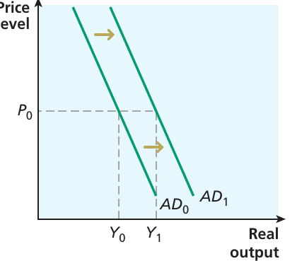
For instance, at price level , real output demanded was initially when the AD curve was at . After government spending increases and the curve shifts to , real output demanded at price level has increased to . The effects of such shifts on the macroeconomy will be explored in detail after we examine aggregate supply in the following chapters.
Critical Distinction: Movements vs Shifts
Always clearly distinguish between movements along the AD curve and shifts of the curve:
Movement along the AD curve:
- Caused by a change in the overall price level
- Results in movement from one point to another on the same curve
- Represents a change in quantity of output demanded due to price changes
Shift of the AD curve:
- Caused by a change in any component of aggregate demand (C, I, G, or X − M)
- The entire curve moves left or right
- At any given price level, the quantity of output demanded has changed
This distinction is critical for correct macroeconomic analysis and will appear frequently in exam questions.
Key Points to Remember:
-
Aggregate demand comprises four components: consumption (C), investment (I), government expenditure (G), and net exports (X − M). The formula shows how these elements combine.
-
Consumption is the largest component of aggregate demand in the UK, accounting for approximately 64% of GDP. It is primarily determined by disposable income, but is also influenced by wealth, interest rates, and consumer confidence. The marginal propensity to consume measures how much of additional income households will spend rather than save.
-
Investment increases the economy's productive capacity and is influenced by expectations about future demand, interest rates, government incentives, and the availability of finance. The distinction between gross investment and net investment is important - net investment represents the true addition to the capital stock after accounting for depreciation.
-
Government expenditure can be largely autonomous in the short run, though automatic stabilisers cause some government spending to vary countercyclically with economic activity. Discretionary fiscal policy allows governments to deliberately adjust spending to influence aggregate demand.
-
The aggregate demand curve slopes downward due to three key effects: the real balance effect (price changes affect purchasing power), the interest rate effect (price changes influence borrowing costs), and the trade effect (price changes affect international competitiveness). Changes in the price level cause movements along the AD curve, while changes in any component of AD cause the entire curve to shift.