Overview (Leaving Cert Applied Maths): Revision Notes
Overview
Dynamic programming is a powerful mathematical technique used to solve complex problems by breaking them down into simpler, manageable stages. This method is particularly useful for making optimal decisions across multiple time periods or steps, where each decision affects future options.
What is dynamic programming?
Dynamic programming works by solving multi-stage decision problems systematically. Instead of trying to solve everything at once, it tackles each stage individually whilst keeping track of the optimal outcomes. This approach helps us find the best possible solution when we need to make a series of connected decisions over time.
The key principle is that each decision made at one stage will influence the available options and outcomes at subsequent stages. By working backwards from the final stage or forwards from the beginning, we can determine the optimal path through all possible decisions.
The four main types of problems
Dynamic programming can be applied to four main categories of problems, each with its own specific characteristics and applications:
1. Routing problems
Routing problems involve finding the optimal path or journey through different locations. These problems focus on minimising costs or maximising profits whilst moving between destinations over a series of stages.
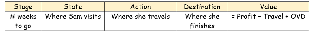
In routing problems, the stage represents the number of time periods remaining (such as weeks), the state shows the current location, the action is the choice of where to travel next, the destination is where you end up, and the value combines profit earned minus travel costs plus any additional factors.
Routing Value Calculation: Value = Profit - Travel + OVD
2. Stock control problems
Stock control problems deal with managing inventory levels over time. These involve decisions about how much to produce, how much to store, and how to balance costs whilst meeting demand.
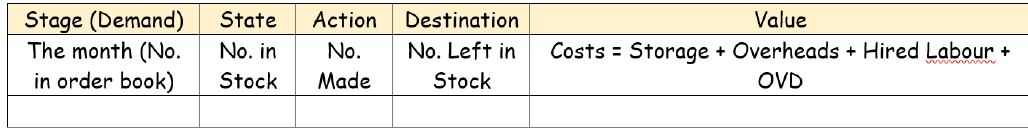
For stock control, the stage represents the time period (typically months with known demand), the state shows current stock levels, the action is how many items to manufacture, the destination is the resulting stock level, and the value includes all associated costs like storage, overheads, and labour.
Stock Control Value Calculation: Costs = Storage + Overheads + Hired Labour + OVD
3. Resource allocation problems
Resource allocation problems focus on distributing limited resources optimally across different uses or projects. The goal is typically to maximise profit or benefit from the available resources.

In resource allocation, the stage represents different products or projects, the state shows the amount of resource currently available (such as tonnes), the action is how much to allocate to this stage, the destination is what remains for future stages, and the value represents the profit generated.
Resource Allocation Value Calculation: Value = Profit + OVD
4. Equipment maintenance problems
Equipment maintenance problems involve decisions about when to replace or maintain equipment to minimise total costs over time. These problems balance the costs of maintenance against the benefits of newer equipment.
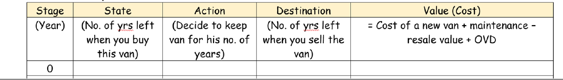
For equipment maintenance, the stage represents the year or time period, the state shows the age of equipment when making a decision, the action is how long to keep the equipment, the destination is the equipment's age when eventually replaced, and the value includes purchase costs, maintenance costs, and resale values.
Equipment Maintenance Value Calculation: Value = Cost of a new van + maintenance - resale value + OVD
Understanding the table structure
All dynamic programming problems use a similar table structure with five key columns:
- Stage: The current step or time period in the decision process
- State: The situation or condition you're in at this stage
- Action: The decision or choice you make at this stage
- Destination: Where this action takes you for the next stage
- Value: The cost or benefit associated with this decision path
Understanding OVD (Optimal Value to Destination)
You'll notice that OVD appears in all value calculations. This represents the optimal value that can be achieved from the destination state onwards. It's calculated by working through the problem systematically and represents the best possible outcome from any given point forwards.
Key benefits of dynamic programming
Dynamic programming offers several advantages for solving complex problems:
- Systematic approach: Breaks down complex problems into manageable pieces
- Optimal solutions: Guarantees finding the best possible answer when used correctly
- Flexibility: Can be applied to many different types of decision problems
- Clear structure: The table format makes it easy to track decisions and outcomes
Exam Strategy
When tackling dynamic programming problems in exams:
- Always set up your table with the correct column headings for the problem type
- Work systematically through each stage
- Pay careful attention to the value calculation formula for each problem type
- Remember that OVD links the stages together
- Check your arithmetic carefully as small errors can compound
Key Points to Remember:
- Dynamic programming solves multi-stage decision problems by breaking them into simpler steps
- The four main types are routing, stock control, resource allocation, and equipment maintenance
- All problems use the same five-column table structure: Stage, State, Action, Destination, Value
- Each problem type has its own specific value calculation formula that includes OVD
- The method guarantees optimal solutions when applied correctly to suitable problems