Routing (Leaving Cert Applied Maths): Revision Notes
Routing
What is routing in dynamic programming?
Routing problems are a type of optimisation challenge where you need to find the best path through a network or sequence of decisions. In dynamic programming, routing involves determining the most efficient way to move between different states (locations or positions) over multiple time periods, whilst maximising benefits or minimising costs.
These problems are particularly useful for real-world scenarios like delivery routes, travel planning, resource allocation, and scheduling decisions where you must consider both immediate costs and future consequences.
Dynamic programming routing problems are excellent for modelling sequential decision-making where each choice affects future options and outcomes. The key insight is that optimal solutions require considering the entire sequence of decisions, not just individual steps.
Understanding the problem structure
Routing problems in dynamic programming are typically organised around several key components that work together to model decision-making over time. The network structure provides a visual framework for understanding how different elements connect and interact.
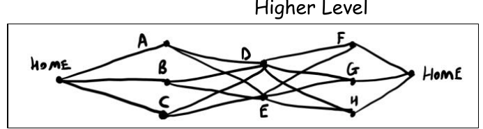
The network structure shows how different locations or states are connected, with possible paths between them. This visual representation helps us understand the relationships and available options at each stage of the decision process.
Problem setup and data organisation
Before solving a routing problem, you need to organise your information into clear data structures. This typically involves three types of information that must be carefully analysed: timing constraints, benefit calculations, and cost analysis.
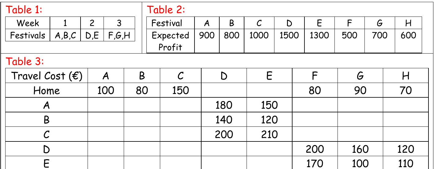
The data organisation includes timing constraints (when certain options are available), benefit calculations (expected returns or profits from each choice), and cost analysis (expenses associated with moving between different states). Understanding how these elements interact is crucial for finding optimal solutions.
Proper data organisation is essential for routing problems. Take time to clearly identify what information represents profits, what represents costs, and what represents constraints or limitations on your decisions.
The backwards approach methodology
Dynamic programming routing problems use a backwards approach, which means you start from the final stage and work backwards to the beginning. This might seem counterintuitive, but it's actually the most logical way to ensure optimal decisions at each step.
Why work backwards?
Working backwards is not just a convention - it's mathematically necessary for optimal solutions:
- You can calculate exact values for future benefits
- Each decision considers all possible future outcomes
- It eliminates uncertainty about what comes next
- It guarantees optimal solutions through systematic analysis
Remember: Start at the END to find the best PATH
Key components of the solution framework
Every routing problem involves five essential elements that form the structure of your solution. Understanding these components is crucial for setting up and solving any routing problem effectively.
Stage - This represents time periods or decision points in your problem. Stages are numbered based on how many time periods remain until the end.
State - These are the possible positions or locations you could be in at each stage. States represent all the viable options available at that point in time.
Action - These are the decisions you can make or the moves you can take from each state. Actions connect your current state to possible future states.
Destination - This shows where each action leads you. The destination becomes your new state in the next stage of the problem.
Value - This is the calculated benefit or cost of taking each action, including both immediate effects and future consequences.
The value calculation formula
The core calculation in routing problems follows a specific pattern that accounts for immediate gains, immediate costs, and future potential. This is the most important formula in routing problems:
The Value Calculation Formula:
Where:
- Profit = Immediate benefit gained from being in that state
- Travel = Cost of moving from current state to destination
- OVD = Optimum Value from Destination (the best possible value you can achieve from where you'll end up)
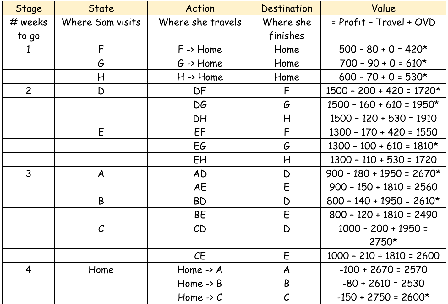
This formula ensures that every decision considers both immediate consequences and future potential.
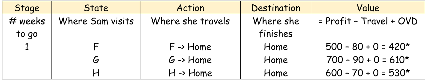
The table shows how this calculation works in practice for the final stage, where OVD equals zero because there are no future stages to consider.
Step-by-step solution process
The solution process involves working through each stage systematically, building up from the final stage to the initial stage. This methodical approach ensures accuracy and completeness.
Worked Example: Solving Routing Problems Step-by-Step
Stage 1 (Final stage):
- Calculate values for all possible final actions using:
- OVD = 0 for all final destinations (no future stages)
- Identify optimal choices (marked with asterisks)
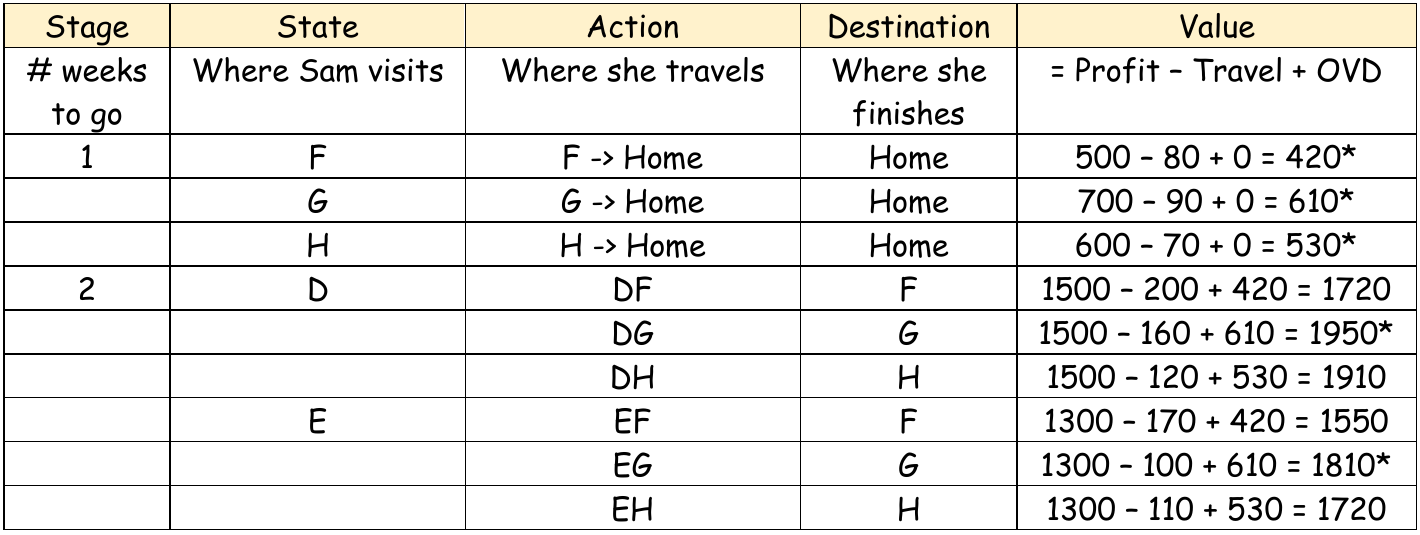
Stage 2 (Previous stage):
- Use optimal values from Stage 1 as OVD inputs
- Calculate values for all possible actions using the full formula
- Identify optimal choices at this stage
Continue backwards through all stages:
- Each stage uses optimal values from the previous calculation
- Build up the complete solution table
- Track optimal paths through asterisk markings
Finding the optimal solution
Once you've completed all stages, the optimal solution can be traced by following the asterisked (optimal) choices from the initial stage through to the final stage. This gives you the sequence of decisions that maximises your overall objective.
The optimal path considers both immediate benefits and long-term consequences, ensuring that short-term decisions don't compromise overall performance. This systematic approach guarantees that you find the truly best solution rather than just a locally optimal one.
When tracing your optimal path, always double-check that you're following the asterisked choices at each stage. The optimal path should form a complete sequence from start to finish with no gaps or inconsistencies.
Practical applications and exam tips
Routing problems appear frequently in Leaving Certificate Applied Mathematics because they demonstrate logical thinking and systematic problem-solving approaches. These skills transfer to many real-world decision-making scenarios.
Exam Success Tips:
- Always start with the final stage - this is crucial for the backwards approach
- Set up your table systematically - use consistent column headings and clear labelling
- Show all calculations - include the profit, travel cost, and OVD components
- Mark optimal solutions clearly - use asterisks or highlighting to identify best choices
- Double-check your OVD values - ensure you're using optimal values from previous stages
Remember that routing problems can apply to many real-world contexts beyond the specific examples you study. The methodology remains consistent whether you're optimising travel routes, resource allocation, investment decisions, or scheduling problems.
Key Points to Remember:
-
Work backwards from the final stage - this ensures optimal decision-making at each step by eliminating uncertainty about future consequences
-
Use the formula consistently for all calculations, remembering that OVD represents the best possible future value from each destination
-
Set up systematic tables with clear columns for Stage, State, Action, Destination, and Value to organise your solution process effectively
-
Mark optimal solutions with asterisks and trace these back to find your complete optimal path from start to finish
-
Final stage OVD is always zero because there are no future stages to consider when calculating terminal values