Introduction to Functions in Spreadsheets (Grade 10 NSC Matric Computer Application Technology): Revision Notes
Introduction to Functions in Spreadsheets
What are functions?
Functions are powerful tools that make spreadsheet calculations much easier and more efficient. Think of a function as a built-in calculator that can perform complex calculations automatically. Unlike simple formulas that use basic operators (+, -, ×, ÷), functions use special reserved words to process your data and produce results.
The key difference between formulas and functions is that formulas perform calculations using operators and individual cell references (like =B3+B4+B5), while functions use predefined procedures to handle entire ranges of data at once (like =SUM(B3:B5)).
Both functions and formulas must always begin with an equals sign (=) to tell the spreadsheet that you want to perform a calculation rather than just enter text.
Understanding function syntax
Every function follows a specific structure called syntax. This is like a recipe that the spreadsheet needs to follow to perform the calculation correctly.
Essential Function Components
The basic syntax of any function includes three essential parts:
- Equals sign (=) - This tells the spreadsheet you're creating a calculation
- Function name - This specifies which type of calculation you want (like SUM, AVERAGE, etc.)
- Arguments - These are the values or cell ranges the function will work with, always enclosed in parentheses
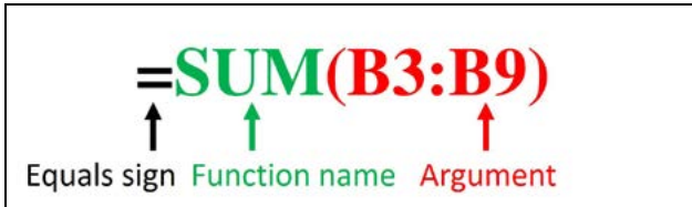
For example, in the function =SUM(B3:B9):
=is the equals sign:coderef[SUM]is the function name(B3:B9)is the argument specifying the range of cells to add
Working with arguments
Arguments are the information that functions need to perform their calculations. Think of them as the ingredients you give to a recipe. Arguments can be individual cells, ranges of cells, or even specific numbers.
Understanding Arguments
When working with arguments, remember these important points:
Cell ranges: A colon (:) creates a reference to a range of cells. For example, =SUM(B5:B11) will add all values from cell B5 to cell B11.
Separating arguments: When a function needs multiple pieces of information, you separate them with commas or semicolons (depending on your regional settings). For instance, if you want to add several different ranges, you would write something like =SUM(C1:C5,D1:D3,E1:E4).
Individual values: You can also use specific numbers as arguments, such as =SUM(10,20,30).
Common function types
Spreadsheet applications offer many different functions, but five are particularly useful for everyday calculations:
| Function | What it does | Example |
|---|---|---|
| SUM | Adds all the values in a range | =SUM(B2:B10) |
| AVERAGE | Calculates the mean (average) of values | =AVERAGE(B2:B10) |
| COUNT | Counts how many cells contain numbers | =COUNT(B2:B10) |
| MIN | Finds the smallest value in a range | =MIN(B2:B10) |
| MAX | Finds the largest value in a range | =MAX(B2:B10) |
These functions are incredibly useful for analysing data quickly without having to write complex formulas.
Worked example: Using the SUM function
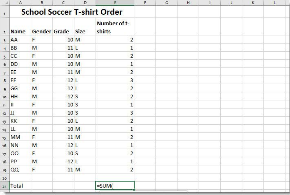
Let's look at a practical example using a school soccer team's t-shirt order data:
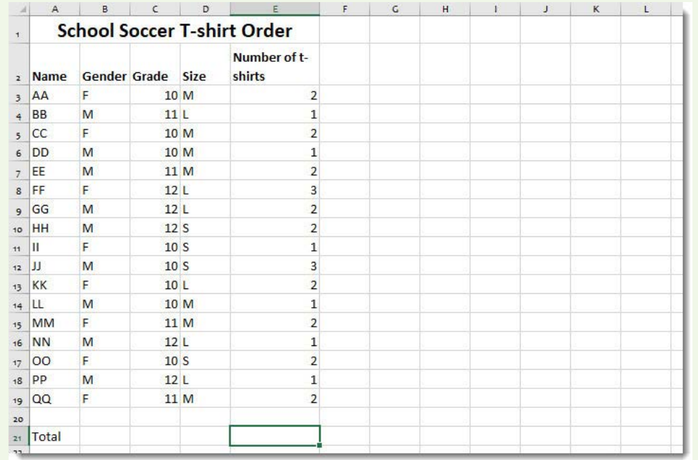
Worked Example: Calculating Total T-Shirts with SUM Function
To calculate the total number of t-shirts needed, we can use the SUM function instead of adding each quantity individually.
Step 1: Click on the cell where you want the total to appear (usually at the bottom of your data).
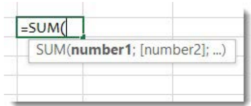
Step 2: Type =SUM( - notice how the spreadsheet provides helpful hints about the function syntax.
Step 3: Select the range of cells containing the quantities you want to add. You can do this by clicking and dragging, or by typing the range directly (like E3
).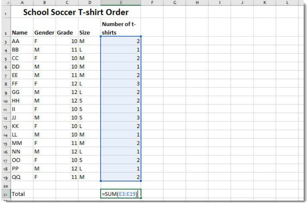
Step 4: Close the parentheses by typing ) and press Enter.
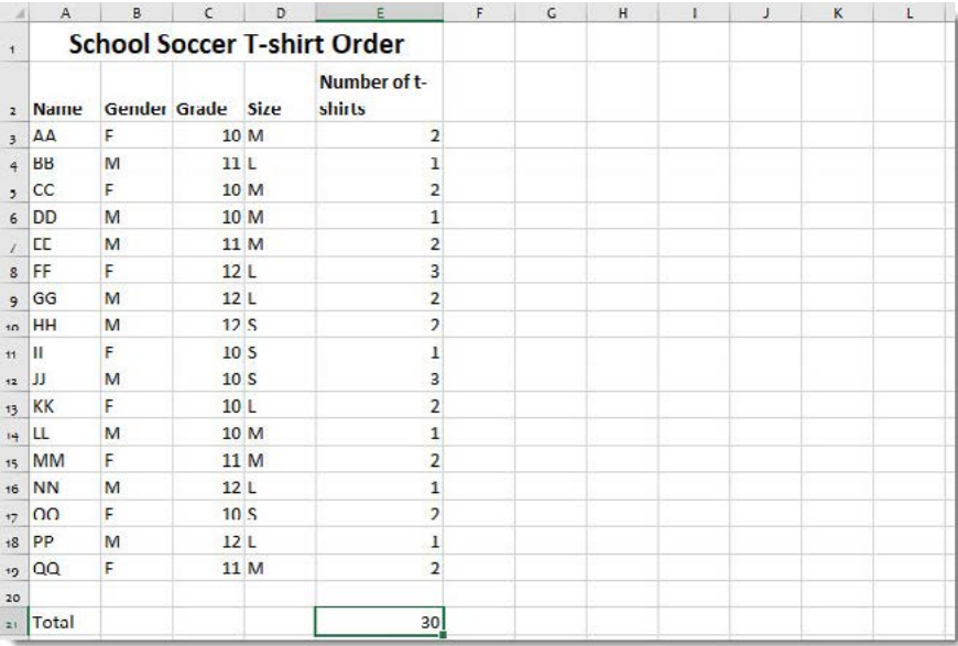
Result: The spreadsheet will automatically calculate the total, which in this example is 30 t-shirts.
Working example: Using the AVERAGE function
Using the same t-shirt order data, we can calculate the average number of t-shirts per student:
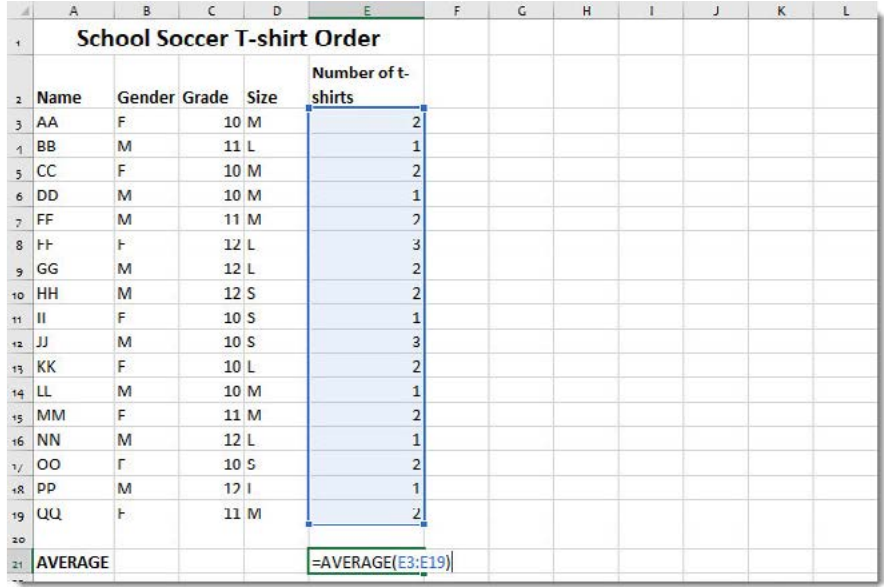
Worked Example: Calculating Average with AVERAGE Function
The process is very similar to using SUM:
- Select the cell where you want the average to appear
- Type
=AVERAGE( - Select the same range of data (E3)
- Close the parentheses and press Enter
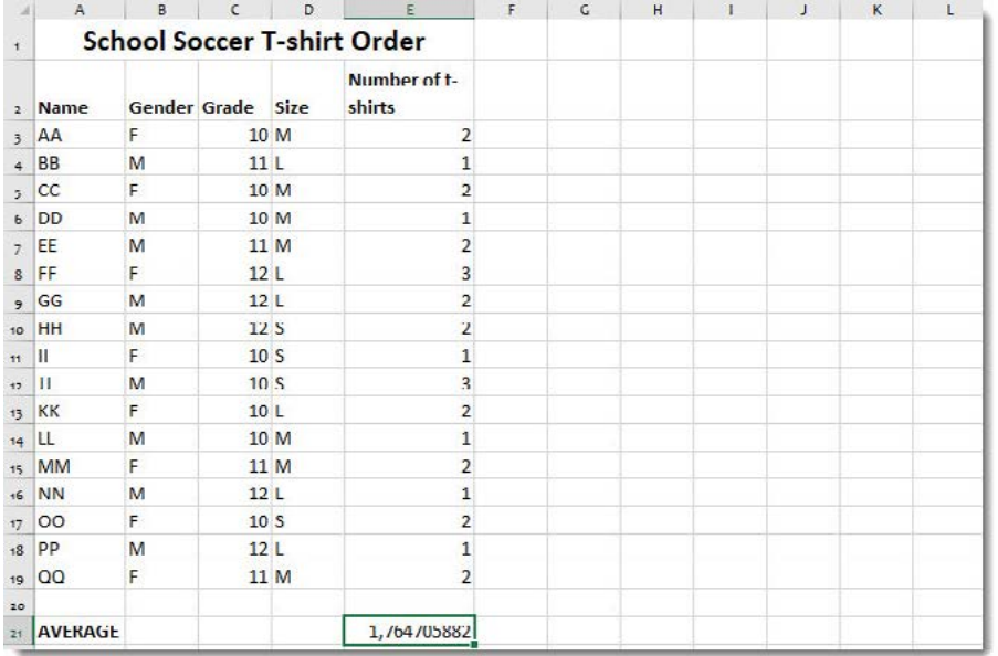
Result: The result shows that on average, each student ordered approximately 1.76 t-shirts.
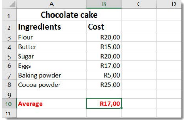
Here's another example using ingredient costs for a chocolate cake:
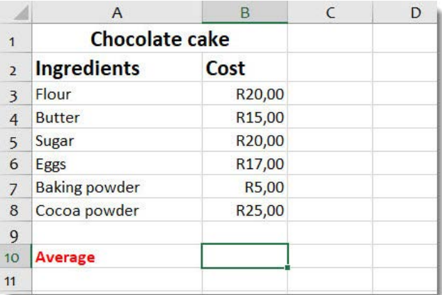
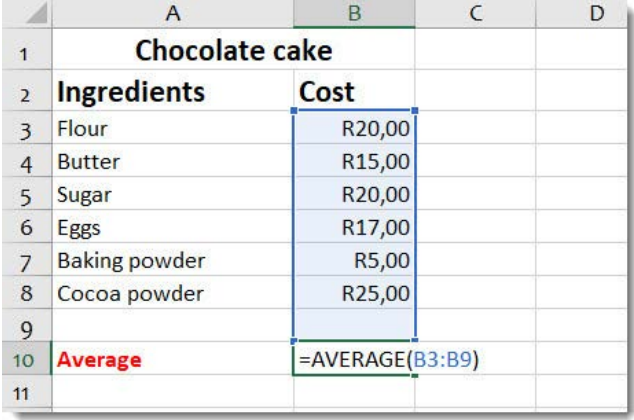
By using =AVERAGE(B3:B9), we can quickly find that the average ingredient cost is R17.00.
Using AutoSum for quick calculations
Time-Saving Feature: AutoSum
AutoSum is a time-saving feature that automatically inserts the most common functions for you. Instead of typing the entire function, you can use AutoSum to insert functions quickly.
To use AutoSum:
- Select the cell where you want your result
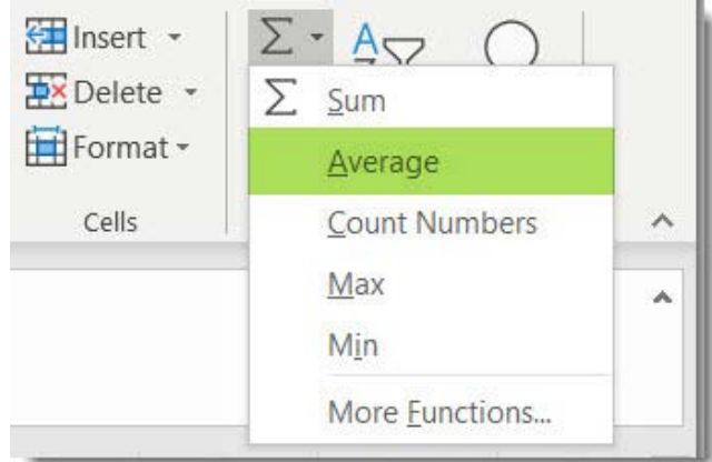
- Look for the AutoSum button (Σ) in your toolbar
- Click the dropdown arrow next to it
- Choose the function you need (Sum, Average, Count Numbers, Max, Min)
- The spreadsheet will automatically suggest a range of cells and insert the function
This method is particularly helpful when you're working with data that's organised in neat columns or rows, as the spreadsheet can usually guess which cells you want to include in your calculation.
Working with multiple arguments
Sometimes you need to perform calculations on several different ranges of cells that aren't next to each other. Functions can handle multiple arguments by separating them with commas or semicolons.
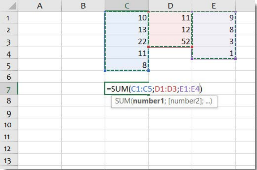
For example, =SUM(C1:C5;D1:D3;E1:E4) will add:
- All values in cells C1 through C5
- All values in cells D1 through D3
- All values in cells E1 through E4
This is much more efficient than creating separate functions and then adding their results together.
Understanding error indicators
When working with functions, you might sometimes see error messages instead of the results you expect. These error indicators help you identify and fix problems with your functions:
Common Function Errors and Solutions
| Error | What it means | How to fix it |
|---|---|---|
| #### | The column is too narrow to display the number | Widen the column by dragging its border |
| #NAME! | You've misspelt the function name | Check the spelling of your function name |
| #DIV/0! | You're trying to divide by zero or an empty cell | Check that your divisor isn't zero or empty |
| #REF! | You're referring to a cell that no longer exists | Update your cell references to valid cells |
| #VALUE! | You're using text where numbers are expected | Make sure your data contains numbers, not text |
| #NUM! | The calculation result is too large or impossible | Check your numbers and calculation logic |
Don't be worried when you see these errors - they're actually helpful diagnostic tools that guide you towards fixing your functions.
Exam tips and strategies
When working with functions in assessments:
- Always start with =: Remember that every function must begin with an equals sign
- Check your parentheses: Make sure every opening parenthesis has a matching closing one
- Verify your ranges: Double-check that your cell ranges include all the data you need
- Use AutoSum when appropriate: It's faster and reduces typing errors
- Read error messages carefully: They often tell you exactly what needs to be fixed
Key Points to Remember:
- Functions are powerful built-in procedures that automate complex calculations
- Every function requires proper syntax: equals sign + function name + arguments in parentheses
- Arguments tell the function which data to work with - they can be individual cells, ranges, or values
- The five most common functions (SUM, AVERAGE, COUNT, MIN, MAX) handle most basic data analysis needs
- AutoSum provides a quick way to insert common functions without typing them manually
- Error indicators are helpful diagnostic tools that guide you towards fixing problems with your functions