Basic Concepts of Spreadsheets (Grade 10 NSC Matric Computer Application Technology): Revision Notes
Basic Concepts of Spreadsheets
What is a spreadsheet?
A spreadsheet is a powerful computer application that helps you organise and work with data using rows and columns. Think of it like a digital table that can perform calculations automatically. The most popular spreadsheet programme is Microsoft Excel, but there are others like Google Sheets and LibreOffice Calc.
When you want to open a spreadsheet programme like Excel, you simply click on the Start button and select the programme from the list. If there's a shortcut on your desktop or taskbar, you can click on that too.
Popular spreadsheet applications include Microsoft Excel (part of Office suite), Google Sheets (free, web-based), LibreOffice Calc (free, open-source), and Apple Numbers (for Mac users). Each has similar core functionality but may have different interface layouts and advanced features.
Understanding workbooks and worksheets
When you work with spreadsheets, you're actually working with something called a workbook. A workbook is like a file that contains one or more worksheets. Each worksheet is a separate page with its own grid of rows and columns where you can enter data.
You can see the different worksheets at the bottom of your screen as tabs (like "Sheet1", "Sheet2", etc.). To switch between worksheets, simply click on the tab you want to work with. This is really handy when you need to organise different types of information separately but keep them in the same file.
Think of a workbook as a binder and worksheets as individual pages in that binder. This organisation allows you to keep related data together while maintaining clear separation between different datasets or calculations.
The basic structure: cells, rows, and columns
The heart of any spreadsheet is its grid structure made up of:
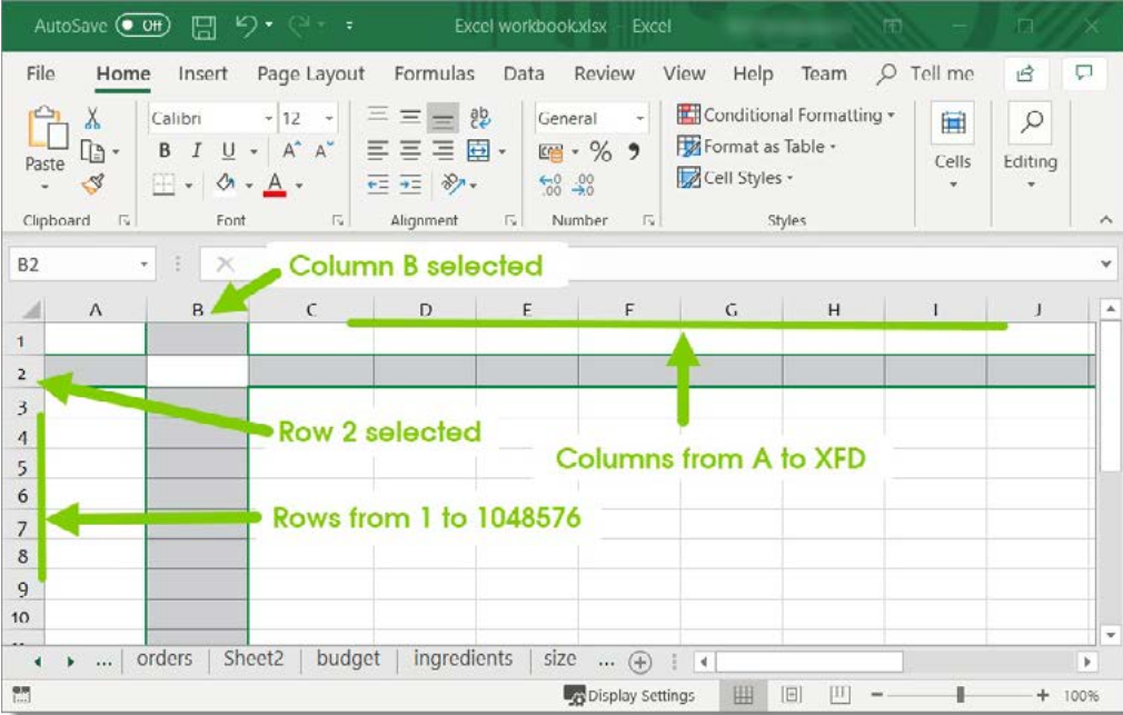
- Columns: These run vertically (up and down) and are labelled with letters (A, B, C, D, etc.). In Excel, you can have columns from A all the way to XFD - that's over 16,000 columns!
- Rows: These run horizontally (left to right) and are numbered (1, 2, 3, 4, etc.). Excel allows up to 1,048,576 rows.
- Cells: Where a column and row meet, you get a cell. This is where you actually enter your data.
Excel's massive capacity of over 16,000 columns and more than 1 million rows means you're unlikely to ever run out of space for your data. However, larger spreadsheets can become slower to work with, so it's good practice to keep your data organised and remove unused areas.
Cell addresses and the name box
Every cell has a unique address, just like houses have street addresses. The cell address combines the column letter with the row number. For example, if you click on the cell where column C meets row 5, that cell's address is C5.
You can always see which cell you've selected by looking at the name box in the top-left corner of the screen. When you select cell C5, you'll see C5 displayed in the name box.
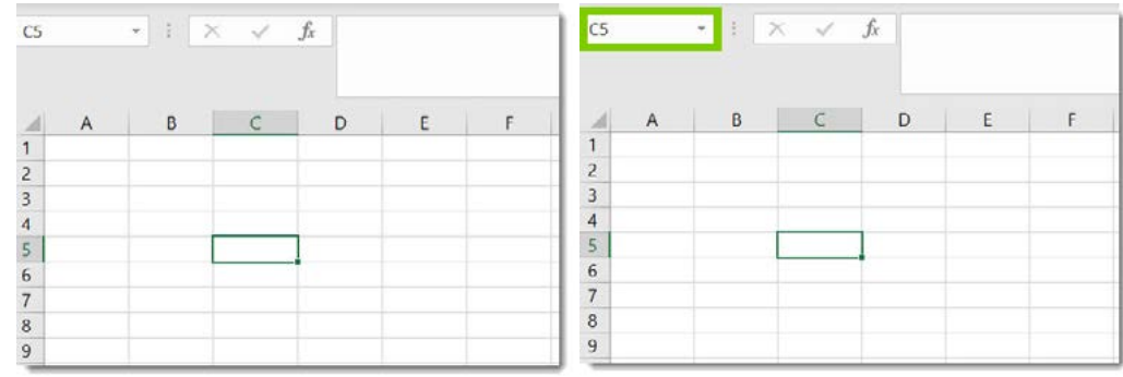
The cell address also appears in the name box, and when a cell is selected, both the column header and row header get highlighted to show you exactly where you are.
The name box isn't just for viewing cell addresses - you can also type a cell address directly into the name box and press Enter to quickly jump to that specific cell, which is especially useful in large spreadsheets.
Understanding the ribbon interface
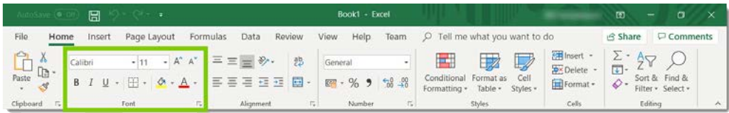
Spreadsheets use a ribbon interface similar to Microsoft Word. The ribbon contains several tabs, and each tab has groups of related commands. You'll use these tabs to perform different tasks in your spreadsheet.
Each tab contains multiple groups of tools. For example, the Home tab includes groups for Font formatting, Alignment, Number formatting, and more. This organised approach makes it easier to find the tools you need.
If you're familiar with other Microsoft Office programmes like Word or PowerPoint, you'll find the ribbon interface very similar. The consistent design across Office applications makes it easier to learn and use different programmes in the suite.
Working with cell ranges
Sometimes you need to work with multiple cells at once. When you select several cells together, this is called a cell range. There are different ways to write cell ranges:
- Single range: If you want to select cells C1, C2, C3, and C4, you write this as C1
- Multiple individual cells: If you want cells that aren't next to each other, you separate them with commas
Understanding cell ranges is important because many spreadsheet functions work on ranges of cells rather than just single cells.
Examples of Cell Range Notation:
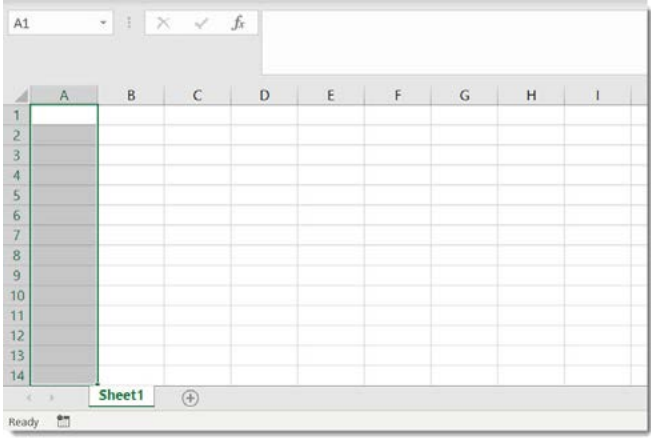
- A1 - selects cells A1 through A10 (a vertical range)
- A1 - selects cells A1 through E1 (a horizontal range)
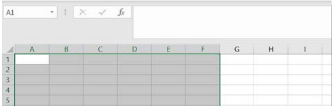
- A1 - selects a rectangular block from A1 to C3
- A1,C3,E5 - selects three individual, non-adjacent cells
Entering data in cells
Getting information into your spreadsheet is straightforward. You simply click on the cell where you want to enter data and start typing. Here are some important points about data entry:
- Text alignment: When you type text into a cell, it automatically aligns to the left side of the cell
- Number alignment: When you enter numbers, they automatically align to the right side of the cell
- Editing cells: To edit what's already in a cell, you can double-click on the cell or click once and then modify the content in the formula bar
The automatic alignment of text and numbers serves a practical purpose - it makes it easier to read columns of data at a glance. Text aligning left and numbers aligning right creates visual consistency that helps you quickly scan and understand your data.
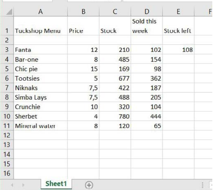
Let's look at a practical example. Imagine you're creating a menu for a school tuckshop. You would enter the item names in one column and their prices in another column. This creates a clear, organised layout that's easy to read and work with.
Introduction to formulas
One of the most powerful features of spreadsheets is their ability to perform calculations automatically using formulas. All formulas in spreadsheets must start with an equals sign (=).
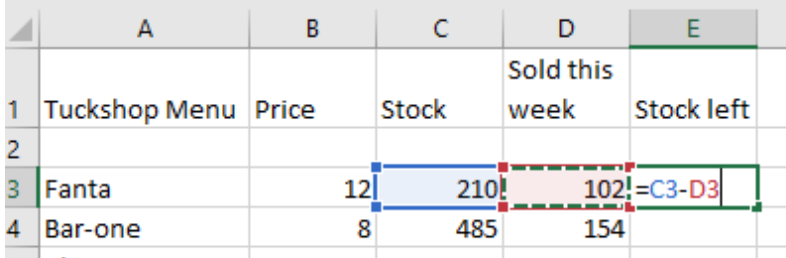
A basic formula might look like this: =C3-D3
Let's break this down:
- = tells the spreadsheet this is a formula
- C3 is the first cell address
- - is the mathematical operator (subtraction)
- D3 is the second cell address
When you enter this formula, the spreadsheet will take the value in cell C3, subtract the value in cell D3, and display the result in the cell where you entered the formula.
Formula Breakdown Example:
If cell C3 contains the value 100 and cell D3 contains the value 25:
Formula: =C3-D3 Calculation: 100 - 25 Result displayed: 75
The power of cell references
Instead of typing actual numbers into your formulas, it's much better to use cell references (the addresses of cells). This means if you change the number in one of the referenced cells, all formulas that use that cell will automatically update.
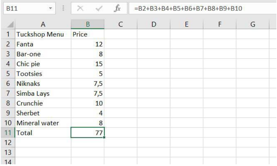
For example, if you have a list of prices and you want to add them up, you could use a formula like =B2+B3+B4+B5+B6+B7+B8+B9+B10. If you later change one of the prices, the total will automatically recalculate.
This automatic updating is one of the biggest advantages of using spreadsheets - you don't have to manually recalculate everything when one number changes.
Always use cell references instead of typing raw numbers into formulas. For example, use =A1*0.15 instead of =100*0.15. This way, if the value in A1 changes, your calculation automatically updates. This principle is fundamental to creating dynamic, maintainable spreadsheets.
Practical application: the tuckshop example
Let's see how all these concepts work together in a real example. Imagine you're managing inventory for a school tuckshop:
You might have columns for:
- Menu items (text data)
- Prices (number data)
- Stock levels (number data)
- Items sold this week (number data)
- Stock remaining (calculated using a formula)
The formula for stock remaining would be: =C3-D3 (original stock minus items sold)
This practical example shows how spreadsheets can help you manage real-world data efficiently.
Complete Tuckshop Inventory Example:
| Item | Price | Original Stock | Sold | Remaining |
|---|---|---|---|---|
| Sandwiches | £2.50 | 50 | 35 | =C2-D2 |
| Fruit Cups | £1.25 | 30 | 18 | =C3-D3 |
| Drinks | £1.00 | 60 | 42 | =C4-D4 |
When you enter these formulas, the "Remaining" column will automatically calculate and display: 15, 12, and 18 respectively.
Remember!
Key Points to Remember:
-
Spreadsheets are organised grids - columns (letters) run vertically, rows (numbers) run horizontally, and cells are where they intersect
-
Every cell has an address - combine the column letter with the row number (like C5) to identify any cell uniquely
-
Workbooks contain worksheets - you can have multiple sheets in one file, each with its own data
-
Formulas start with equals - use = to tell the spreadsheet you're creating a calculation, not just entering text
-
Cell references are powerful - using cell addresses in formulas (like =A1+B1) means your calculations update automatically when the data changes