Formatting Cells: Some Basics (Grade 10 NSC Matric Computer Application Technology): Revision Notes
Formatting Cells: Some Basics
When working with spreadsheets, formatting can completely transform how your data looks and feels. Good formatting makes your worksheet easier to read, more professional, and helps important information stand out. Think of it like decorating your room - the furniture (your data) is there, but the right colours, styles and arrangement make it much more appealing and functional.
Cell borders and shading
Adding colour and borders to cells works just like it does in word processing programmes. These visual elements help separate different sections of your data and draw attention to important information like headings or totals.
Applying background colours to cells
The most basic way to format cells is by adding background colours, also called fill colours. This is particularly useful for header rows or to highlight specific data categories.
To add a background colour, you need to select the cells you want to format first, then access the formatting options through the Home tab. Look for the Fill Colour tool, which appears as a paint bucket icon. When you click on it, you'll see a colour palette with standard colours, theme colours, and options for custom colours.
Sometimes the background colour you choose might make your text hard to read. If this happens, you'll need to either change the text colour or select a different background colour that provides better contrast.
Fill effects
Beyond simple solid colours, spreadsheets offer more sophisticated background options called fill effects. These can add visual interest to your worksheets whilst maintaining professionalism.
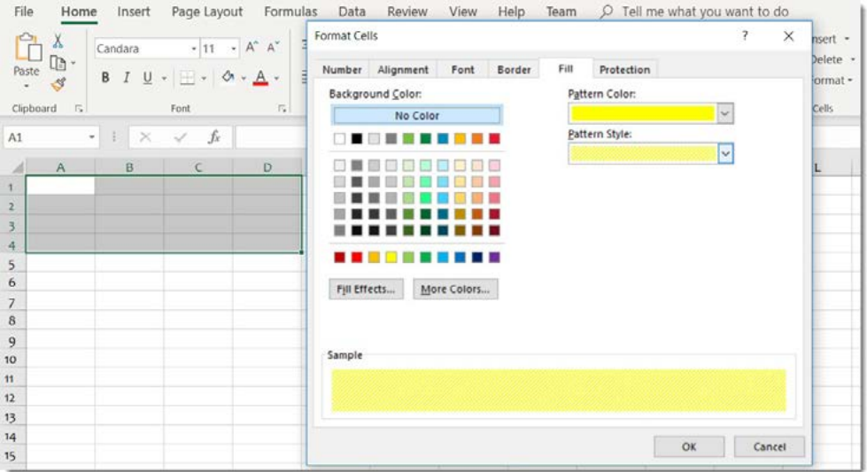
Pattern fills
Pattern fills allow you to add textured backgrounds to cells using combinations of colours and patterns. You can choose from various pattern styles like diagonal stripes, dots, or crosshatches.
When applying patterns, you select both a background colour and a pattern colour. The pattern colour appears over the background colour in the style you choose.
Pattern Fill Example: Creating a Header
Step 1: Select your header cells
Step 2: Choose yellow as your background colour
Step 3: Select diagonal stripes as your pattern
Step 4: Choose blue as your pattern colour
Result: Yellow background with blue diagonal stripes creating a distinctive header appearance.
Gradient fills
Gradient fills create smooth colour transitions within cells, moving from one colour to another. This creates a more sophisticated appearance than solid colours.
With gradients, you typically choose two colours and a shading style. The gradient can move horizontally, vertically, or diagonally across the cell. Popular combinations include moving from light to dark versions of the same colour, or transitioning between complementary colours.
Adding cell borders
Borders help define the structure of your data by creating clear boundaries around cells. They're essential for creating professional-looking tables and separating different sections of information.
The border options include different line styles (solid, dashed, dotted), line weights (thin, medium, thick), and colours. You can apply borders to individual sides of cells or all sides at once.
When working with borders, you have several preset options to choose from:
- None: Removes all borders
- Outline: Adds borders around the outside edges of selected cells
- Inside: Adds borders between cells within your selection
You can also create custom border combinations by selecting specific sides of cells and applying different border styles to each side. This gives you complete control over your table's appearance.
Cell styles
Rather than formatting cells manually each time, spreadsheets provide predefined cell styles that apply multiple formatting options at once. These styles ensure consistency across your worksheet and save time.
Cell styles combine elements like font formatting, borders, fill colours, and alignment into packages that you can apply with a single click. They're particularly useful for headers, titles, and data categories because they maintain a professional, coordinated appearance.
The available styles are often linked to your document's theme colours, which means they'll automatically coordinate with other formatting in your workbook. If you change the theme, the cell styles update accordingly to maintain visual harmony.
When you apply a cell style, it overrides most individual formatting you've done previously, except for text alignment. If you've spent time on detailed formatting, applying a cell style might undo that work.
Text alignment
By default, text in spreadsheet cells aligns to the bottom-left, whilst numbers align to the bottom-right. However, you can control exactly how content appears within cells by changing both horizontal and vertical alignment.
Understanding alignment options
Alignment has two components:
- Horizontal alignment: Controls left-to-right positioning (left, centre, right)
- Vertical alignment: Controls top-to-bottom positioning (top, middle, bottom)
These can be combined in various ways to achieve the exact positioning you want. For example, you might centre text both horizontally and vertically within a cell to create a perfectly centred heading.
Common alignment combinations
Different alignment combinations serve different purposes:
| Vertical | Horizontal | Best Used For |
|---|---|---|
| Top | Left | Standard data entry |
| Top | Centre | Column headings |
| Top | Right | Right-aligned numbers |
| Centre | Left | Row labels |
| Centre | Centre | Titles and emphasis |
| Centre | Right | Right-aligned totals |
| Bottom | Left | Default text position |
| Bottom | Centre | Footer information |
| Bottom | Right | Default number position |
The alignment you choose affects how your data appears and how professional your worksheet looks. Consistent alignment across similar types of data creates a clean, organised appearance.
Formatting columns and rows
Sometimes the default column width or row height doesn't accommodate your data properly. Learning to adjust these dimensions and manage column and row visibility is essential for creating functional worksheets.
Resizing columns and rows
When column content is too wide for the current column width, you'll see symbols like ##### or text that gets cut off. This indicates you need to make the column wider.
The easiest way to resize a column is to position your mouse pointer on the border between column headers until it becomes a double-headed arrow, then drag to adjust the width. You can do the same with row heights by dragging the borders between row numbers.
For more precise control, you can right-click on column or row headers and select specific width or height values. This is useful when you need multiple columns to be exactly the same size.
Multiple column and row adjustments
You can resize several columns or rows simultaneously by selecting multiple headers before dragging. This ensures consistent sizing across your selection.
Selecting Multiple Columns for Resizing:
Step 1: Click and drag across the column letters or row numbers
Step 2: Hold Ctrl and click individual headers to select non-adjacent ones
Step 3: Double-click on column borders to auto-fit the width to the content
Hiding and showing columns and rows
Sometimes you need to temporarily hide certain columns or rows without deleting them. This is useful when you want to focus on specific data or when printing selected portions of your worksheet.
To hide columns or rows, right-click on the header and select Hide from the context menu. Hidden columns and rows don't display, but their data remains intact and continues to be included in calculations.
To unhide hidden columns or rows, select the columns or rows on either side of the hidden section, then right-click and select Unhide. You can also double-click on the border where the hidden section should appear.
Inserting and deleting columns and rows
Adding or removing entire columns and rows is common when your data structure changes. The spreadsheet automatically adjusts cell references in formulas when you insert or delete columns and rows.
When inserting, new columns appear to the left of your selection, and new rows appear above your selection. When deleting, remember that you're removing entire columns or rows, not just the visible content.
It's important to understand the difference between deleting entire rows or columns versus just clearing the content. Deleting removes the structural elements completely, whilst clearing content just empties the cells.
Managing cell contents
If you only want to remove the content from cells without deleting the entire row or column structure, use Clear Contents instead of Delete. This maintains your worksheet structure whilst removing just the data you no longer need.
Key Points to Remember:
- Cell formatting improves readability and creates professional-looking spreadsheets that communicate information effectively
- Fill effects include solid colours, patterns, and gradients - choose options that enhance rather than distract from your data
- Borders help define data structure and create clear visual boundaries between different sections
- Text alignment combines horizontal and vertical positioning to control exactly how content appears within cells
- Column and row management includes resizing, hiding/showing, and inserting/deleting to accommodate your data needs