Advanced Functions (Grade 12 NSC Matric Computer Application Technology): Revision Notes
Advanced Functions
Introduction to advanced functions
Spreadsheet programmes like Excel provide powerful tools that go far beyond basic calculations. Advanced functions allow you to analyse data quickly and efficiently, making it easier to interpret information, make informed decisions, and answer complex questions. These sophisticated tools can handle multiple conditions simultaneously and search through large datasets to find exactly what you're looking for.
Advanced functions are essential for data analysis because they can process complex logic and large datasets in ways that would be time-consuming or impossible with basic formulas alone.
The key advanced functions we'll explore include:
- Complex functions such as nested IF statements and lookup functions
- Error handling techniques to manage issues like #N/A errors
- Variations of familiar functions with enhanced capabilities
- Subtotal and outline features for data organisation
Complex functions
Complex functions enable you to analyse data more thoroughly by combining multiple conditions and operations within a single formula. This approach saves time and reduces errors compared to using multiple separate formulas.
When working with complex functions, always plan your logic carefully before writing the formula. Consider all possible conditions and outcomes to avoid unexpected results.
Nested IF functions
The standard IF function evaluates a single condition and returns one result if true and another if false. However, real-world scenarios often require checking multiple conditions. This is where nested IF functions become invaluable.
A nested IF function places one IF statement inside another, creating a hierarchy of conditions that are evaluated in sequence. The basic structure follows this pattern: the first condition is checked, and if it's true, the corresponding result is returned. If false, the formula moves to the next nested IF condition.
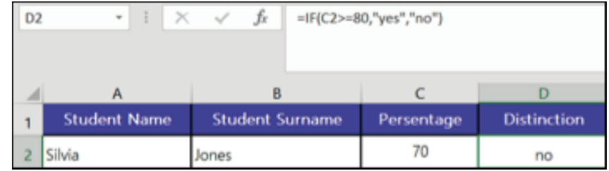
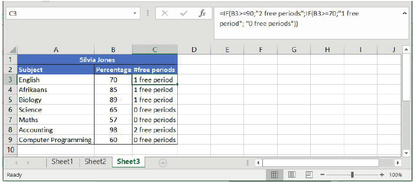
The formula shown demonstrates a simple IF function: =IF(C2>=90,"yes","no"). This checks whether a student's percentage is 90 or above to determine if they receive a distinction. However, what if you need to check multiple grade boundaries?
Worked Example: Multi-Level Grading System
Consider a scenario where a school awards free periods based on academic performance:
- Students scoring 90% or above receive 2 free periods
- Students scoring between 70% and 89% receive 1 free period
- Students scoring below 70% receive 0 free periods
To handle this, you would use a nested IF function:
This formula first checks if the percentage is 90 or above. If true, it returns "2 free periods". If false, it moves to the nested IF function, which checks if the percentage is 70 or above.
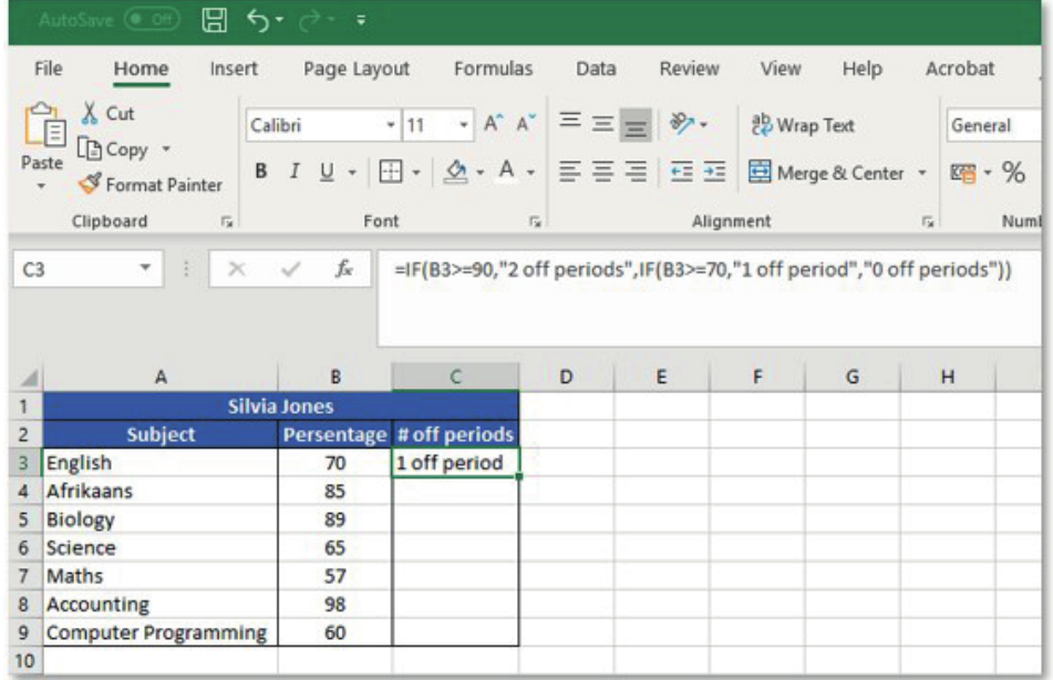
This creates a logical flow that handles all possible grade ranges efficiently.
Using the Insert Function feature
Rather than typing complex formulas manually, Excel provides an Insert Function tool that guides you through the process step by step. This feature is particularly helpful when working with advanced functions that have multiple arguments.
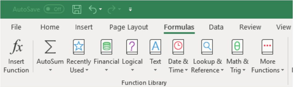
To access this feature:
- Select the cell where you want to insert the function
- Navigate to the Formulas tab in the ribbon
- Click the Insert Function button (fx icon)
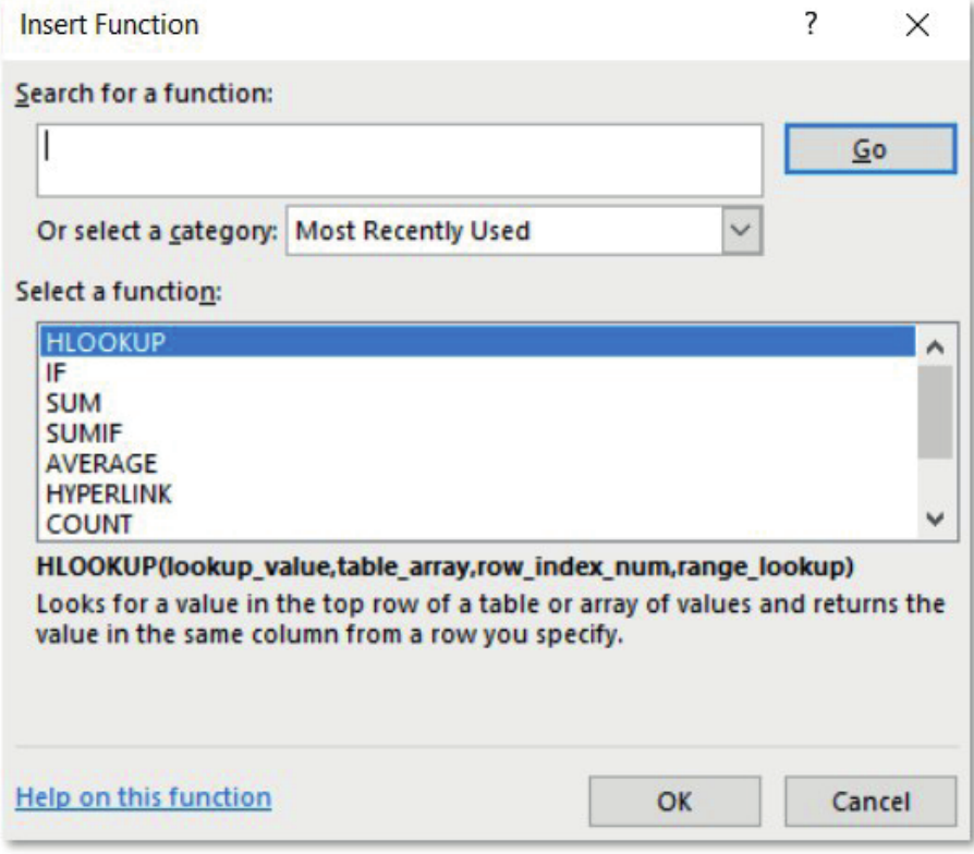
The Insert Function dialogue box opens, allowing you to:
- Search for specific functions by typing keywords
- Browse functions by category (Most Recently Used, Financial, Logical, etc.)
- View detailed descriptions of each function's purpose and syntax
When you select a function and click OK, Excel opens the Function Arguments dialogue, which provides input fields for each required argument. This visual approach helps ensure you enter the correct information in the proper format.
Step-by-step process for creating advanced functions
Worked Example: Creating a Nested IF Function
Let's walk through creating a nested IF function using the Insert Function feature:
- Select your target cell - Choose where you want the formula result to appear
- Open Insert Function - Click the fx button in the Formulas ribbon
- Find your function - Search for "IF" or select it from the Logical category
- Enter the logical test - Input your condition (e.g., B2="rainy")
- Specify true and false values - Enter what should happen for each outcome
- Add nested conditions - For additional IF statements, click in the value_if_false field and insert another IF function
- Review and confirm - Check your formula logic before clicking OK
This systematic approach reduces errors and helps you understand how each part of the formula contributes to the final result.
Lookup functions
When working with large datasets, you often need to find specific information quickly. Lookup functions are designed for exactly this purpose - they search through data systematically and return related information from the same row or column.
Lookup functions are among the most powerful tools in spreadsheet applications, enabling you to work with databases containing thousands of records efficiently.
VLOOKUP (Vertical lookup)
The VLOOKUP function searches for information by looking vertically down the first column of a specified range until it finds a match, then returns a value from a different column in the same row.
The VLOOKUP function consists of four essential components:
| Component | Description | Example |
|---|---|---|
| Lookup_value | The value you're searching for | "Neron McCaffery" |
| Table_array | The range containing your data | A2 |
| Col_index_num | Which column to return data from | 2 (for the second column) |
| Range_lookup | Exact match (FALSE) or approximate (TRUE) | FALSE |
The syntax is:
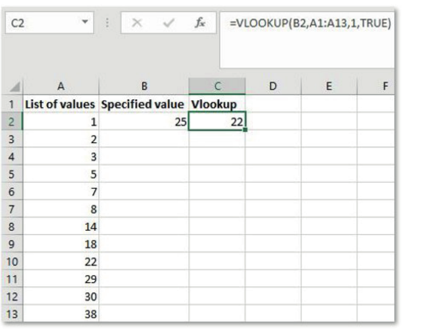
Worked Example: Finding Customer Email
In this example, the formula =VLOOKUP(B2,A1:A13,1,TRUE) searches for the value in cell B2 (which is 25) within the range A1
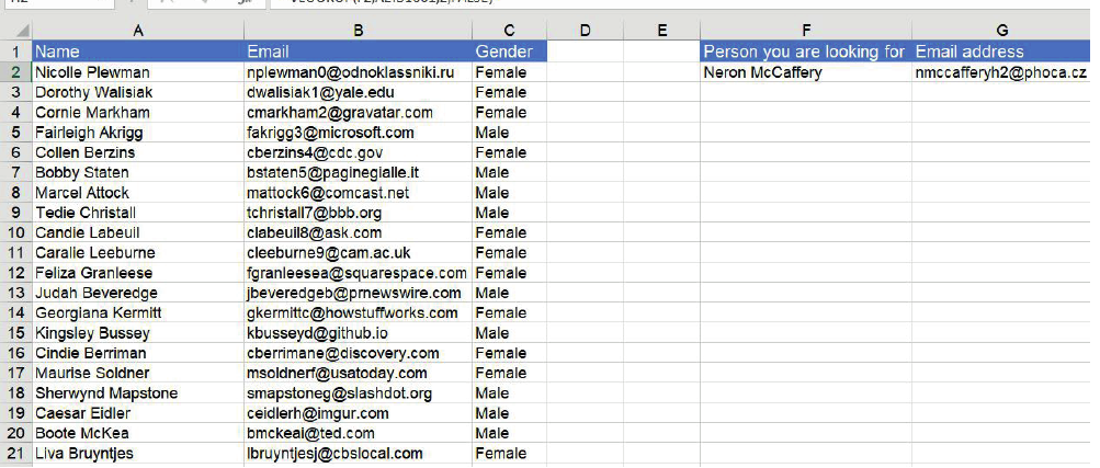
For practical applications, imagine you have a customer database with names and email addresses. Using VLOOKUP, you can quickly find someone's email by searching for their name:
This formula looks for "Neron McCaffery" in the first column and returns the corresponding email address from the second column.
HLOOKUP (Horizontal lookup)
HLOOKUP works similarly to VLOOKUP but searches horizontally across the top row of your data range instead of vertically down the first column. This function is particularly useful when your data is organised in rows rather than columns.
The HLOOKUP function uses these components:
- Function name: HLOOKUP
- Lookup value: The item you're searching for
- Table array: The range containing your data arranged horizontally
- Row index number: Which row contains the data you want to return
- Range lookup: TRUE for approximate match, FALSE for exact match
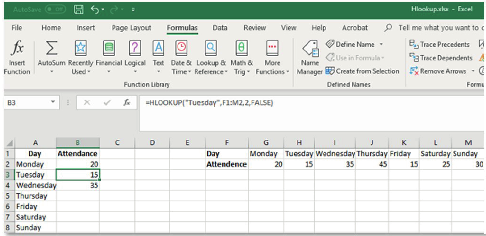
Worked Example: Daily Schedule Lookup
For example: =HLOOKUP("Tuesday",F1:M2,2,FALSE) searches for "Tuesday" in the first row of the range F1
Practical applications
Real-World Applications
Lookup functions are invaluable in real-world scenarios:
- Student records: Finding grades for specific students in large class lists
- Inventory management: Looking up product prices or stock levels
- Employee databases: Retrieving contact information or salary details
- Sales analysis: Finding performance data for specific time periods or regions
The key to using lookup functions effectively is understanding your data structure and choosing the appropriate function (VLOOKUP for column-oriented data, HLOOKUP for row-oriented data) with the correct match type (exact or approximate).
Always specify exact match (FALSE) unless you specifically need approximate matching, as this prevents unexpected results from partial matches.
Key Points to Remember:
- Nested IF functions allow you to test multiple conditions in a single formula, making complex decision-making more efficient
- The Insert Function feature guides you through creating formulas step by step, reducing errors and helping you understand function syntax
- VLOOKUP searches vertically down columns - use it when your lookup data is arranged in columns with the search criteria in the leftmost column
- HLOOKUP searches horizontally across rows - use it when your lookup data is arranged in rows with search criteria in the top row
- Always specify exact match (FALSE) unless you specifically need approximate matching, as this prevents unexpected results from partial matches