More Advanced Functions (Grade 12 NSC Matric Computer Application Technology): Revision Notes
More Advanced Functions
Advanced functions in spreadsheets help you perform complex calculations and data analysis tasks that go beyond basic arithmetic. These functions allow you to combine multiple conditions, handle errors gracefully, and create sophisticated reports from your data.
Logical functions (AND/OR)
Logical functions help you test multiple conditions at the same time and return TRUE or FALSE based on whether those conditions are met. These are particularly useful when you need to philtre data or make decisions based on several criteria.
Boolean logic is fundamental to spreadsheet analysis. Understanding how TRUE and FALSE values work will help you create more sophisticated formulas and data analysis.
The AND function
The AND function checks if ALL specified conditions are true. It only returns TRUE when every single condition you specify is met. If even one condition is false, the entire function returns FALSE.
Function Syntax: AND
=AND(condition1, condition2, condition3, ...)
Example: Job Application Screening To identify female applicants who are 18 years or older:
=AND(A2="Female", B2>=18)
This formula checks both conditions:
- The person must be female (A2="Female")
- The person must be 18 or older (B2>=18)
Only when both conditions are true will the function return TRUE.
The OR function
The OR function checks if AT LEAST ONE of the specified conditions is true. It returns TRUE when any one (or more) of your conditions is met, and only returns FALSE when all conditions are false.
Function Syntax: OR
=OR(condition1, condition2, condition3, ...)
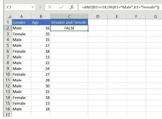
Combined Logic Example
=AND(B2>=18, OR(A2="Male", A2="Female"))
This formula checks that someone is 18 or older AND is either male or female. The OR part ensures the gender field contains valid data.
Error indicators
Excel displays various error indicators when something goes wrong with your formulas. Understanding these errors helps you identify and fix problems in your spreadsheets.
The #N/A error
The #N/A error appears when a function cannot find the value it's been asked to locate. This commonly happens with LOOKUP functions when:
- You're looking for data that doesn't exist in your dataset
- There's a spelling mistake in the lookup value
- You've specified an incorrect cell range that doesn't contain the value you're searching for
To avoid #N/A errors, always double-check that your lookup values exist in your data range and that you've referenced the correct cells.
Rounding function variations
The ROUND function family helps you control how decimal numbers are displayed and calculated in your spreadsheets. This is essential for financial calculations and data presentation.
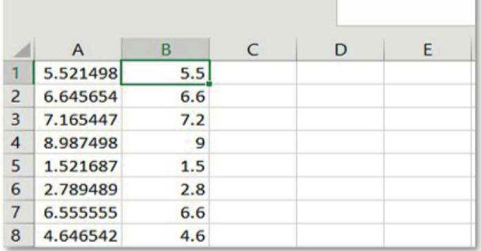
ROUND function
The standard ROUND function rounds numbers using normal mathematical rules - values of 0.5 and above round up, while values below 0.5 round down.
Function Syntax: ROUND
=ROUND(number, decimal_places)
- number: The value you want to round
- decimal_places: How many decimal places you want (use 0 for whole numbers)
ROUNDUP and ROUNDDOWN functions
Sometimes you need more control over rounding direction, regardless of the decimal value.
Directional Rounding Functions
ROUNDUP always rounds numbers towards the higher value:
=ROUNDUP(number, decimal_places)
ROUNDDOWN always rounds numbers towards the lower value:
=ROUNDDOWN(number, decimal_places)
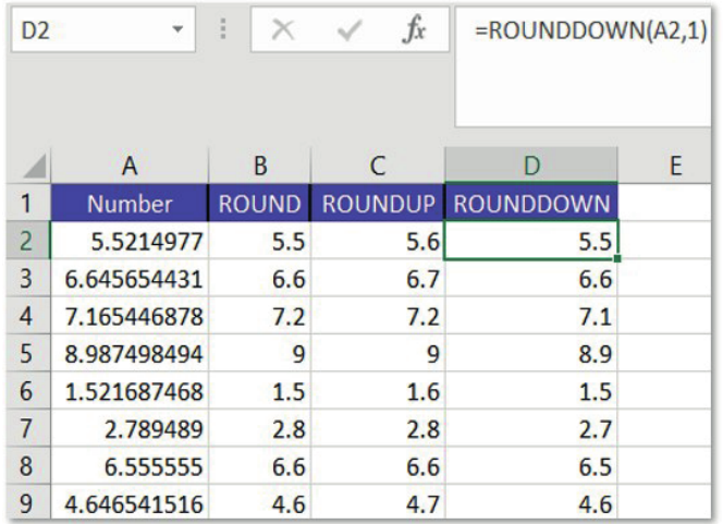
These functions are particularly useful in business situations where you need consistent rounding behaviour, such as always rounding up prices or always rounding down inventory calculations.
Conditional sum and count functions
These powerful functions allow you to perform calculations only on data that meets specific criteria. They're essential for data analysis and creating meaningful reports from large datasets.
SUMIF function
SUMIF adds up values in a range, but only includes cells that meet a specific condition. This is perfect for calculating totals for specific categories or criteria.
Function Syntax: SUMIF
=SUMIF(range, criteria, sum_range)
- range: The cells to check for your criteria
- criteria: The condition that must be met
- sum_range: The cells to add up (if different from the range being checked)
Example: Calculate Total Sales for Vodacom
=SUMIF(B2:B10, "Vodacom", C2:C10)
This formula looks at the provider column (B2
), finds all cells containing "Vodacom", and adds up the corresponding costs from column C.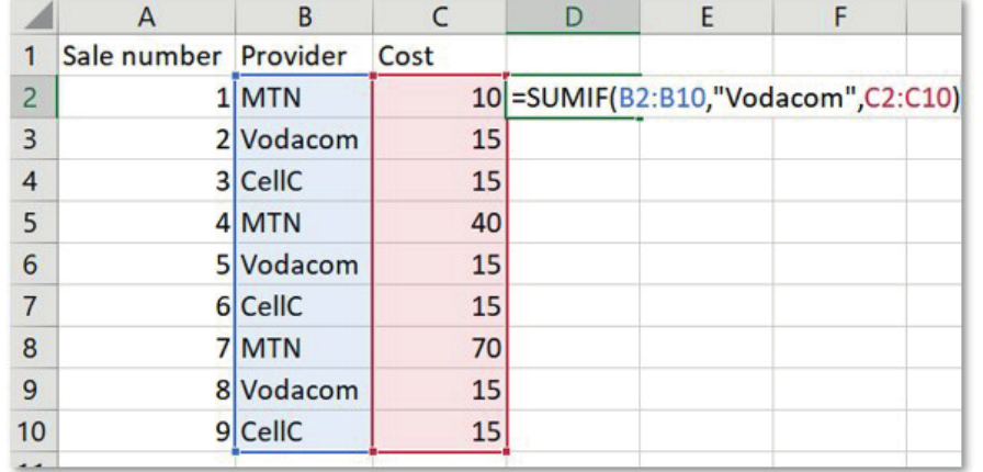
COUNTIF function
COUNTIF counts how many cells in a range meet a specific condition. This helps you analyse the frequency of different values in your data.
Function Syntax: COUNTIF
=COUNTIF(range, criteria)
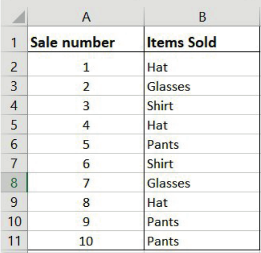
Example: Count Product Occurrences To count how many times "Hat" appears in a sales list:
=COUNTIF(B2:B11, "Hat")
SUMIFS and COUNTIFS functions
When you need to check multiple criteria simultaneously, use the "S" versions of these functions.
Function Syntax: SUMIFS
=SUMIFS(sum_range, criteria_range1, criteria1, criteria_range2, criteria2, ...)
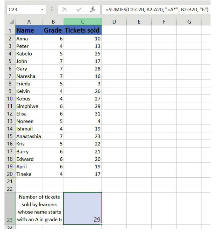
Example: Multiple Criteria Sum Sum tickets sold by students whose names start with "A" and are in grade 6:
=SUMIFS(C2:C20, A2:A20, "A*", B2:B20, "6")
Function Syntax: COUNTIFS
=COUNTIFS(criteria_range1, criteria1, criteria_range2, criteria2, ...)
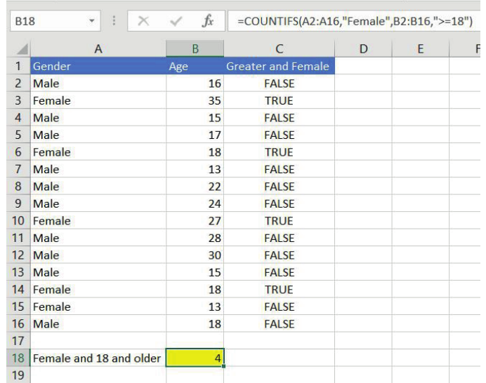
Example: Multiple Criteria Count Count females aged 18 and older:
=COUNTIFS(A2:A16, "Female", B2:B16, ">=18")
Subtotal outline feature
The Subtotal feature automatically creates groups in your data and calculates summary statistics for each group. This is incredibly useful for creating reports that show totals by category, region, or any other grouping field.
How subtotals work
The Subtotal feature provides several powerful capabilities:
- Automatically groups your data by a chosen field
- Calculates functions like SUM, COUNT, AVERAGE, MIN, or MAX for each group
- Creates collapsible outline levels so you can expand or collapse groups
- Adds a grand total at the bottom
Using the subtotal feature
Steps to Create Subtotals
- First, sort your data by the field you want to group by (e.g., by country or category)
- Select your data range
- Go to the Data tab and click Subtotal in the Outline group
- Choose your grouping field and the function you want to calculate
- Select which columns should have subtotals calculated
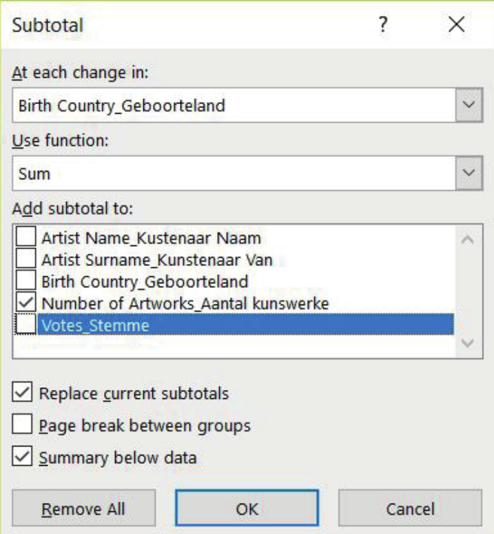
The result is a structured report with subtotals for each group and a grand total:
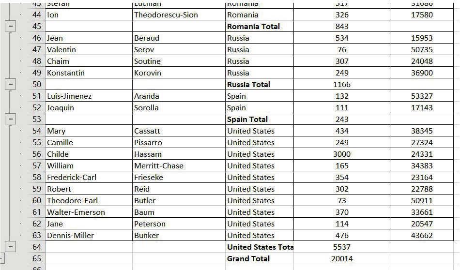
Exam tips and common pitfalls
Critical Points to Remember
When working with advanced functions, remember these important points:
- Check your cell references: Ensure ranges include all necessary data but don't include headers unless intended
- Use absolute references ($ symbols) when copying formulas to prevent ranges from shifting incorrectly
- Quote text criteria: Always put text conditions in quotation marks (e.g., "Vodacom", "Female")
- Test with simple data: Try your formulas on small, known datasets before applying to large spreadsheets
- Watch for case sensitivity: "vodacom" and "Vodacom" are different - ensure consistent capitalisation
- Use wildcards carefully: "*" matches any characters, "?" matches single characters
Key Points to Remember:
- AND requires ALL conditions to be true; OR needs only ONE condition to be true
- #N/A errors usually mean your lookup value doesn't exist in the data range
- ROUND follows normal maths rules, but ROUNDUP and ROUNDDOWN always go in their named direction
- SUMIF/COUNTIF work with single criteria; add an "S" (SUMIFS/COUNTIFS) for multiple criteria
- Subtotals automatically group and summarise data, making professional reports easy to create