Output Profit and Loss (Grade 12 NSC Matric Economics): Revision Notes
Output Profit and Loss
In imperfect markets like monopolies, understanding how businesses determine their output levels and whether they make profits or losses is crucial for economic analysis. Unlike perfectly competitive markets, monopolists have the power to influence both price and quantity, which creates unique patterns in their revenue, costs, and profit outcomes.
Revenue concepts for monopolists
A monopolist faces a very different demand situation compared to perfectly competitive firms. The key to understanding monopoly behaviour lies in grasping how their revenue curves work.
The demand curve and average revenue
For a monopolist, the demand curve represents the market demand curve, which slopes downwards from left to right. This downward slope is fundamental because it means the monopolist cannot sell unlimited quantities at a fixed price. Instead, to sell more units, the monopolist must lower the price for all units sold.
The demand curve is also the average revenue (AR) curve for the monopolist. Average revenue is calculated by dividing total revenue by the quantity sold, which equals the price. Any point on the demand curve represents both a price-quantity combination and the average revenue for that level of output.
Average revenue formula:
Where AR = Average Revenue, TR = Total Revenue, Q = Quantity, and P = Price
Marginal revenue relationship
The marginal revenue (MR) curve shows the additional revenue earned from selling one more unit. For monopolists, the MR curve always lies below the demand (AR) curve. This happens because when a monopolist wants to sell an additional unit, they must reduce the price not just for that extra unit, but for all units sold.
Critical relationship: For monopolists, the MR curve always lies below the demand (AR) curve. This is a fundamental difference from perfectly competitive markets where MR = AR = P.
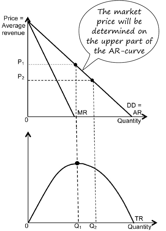
The MR curve intersects the horizontal axis at a point halfway between the origin and where the demand curve meets the horizontal axis. This relationship is mathematically consistent and helps explain why monopolists behave differently from competitive firms.
Total revenue maximisation
The total revenue (TR) curve shows the relationship between output levels and total income. This curve has an inverted U-shape, starting at zero, rising to a maximum point, then declining. The monopolist will try to set prices in the upper part of the demand curve because this is where total revenue increases with higher prices.
The maximum point on the total revenue curve occurs where marginal revenue equals zero. Beyond this point, additional sales actually reduce total revenue because the price cuts needed to sell extra units are so large that they offset the revenue from additional sales.
Economic profit in the short term
Understanding how monopolists maximise profits requires combining their revenue curves with their cost structures. The profit-maximising output occurs where marginal cost equals marginal revenue.
Step-by-step approach to profit maximisation
Worked Example: Drawing Profit Maximisation Graphs
Step 1: Drawing the basic framework Begin by drawing your coordinate system with Price on the vertical axis and Quantity on the horizontal axis. These axes should meet at the origin (0), and everything should be clearly labelled for accurate analysis.
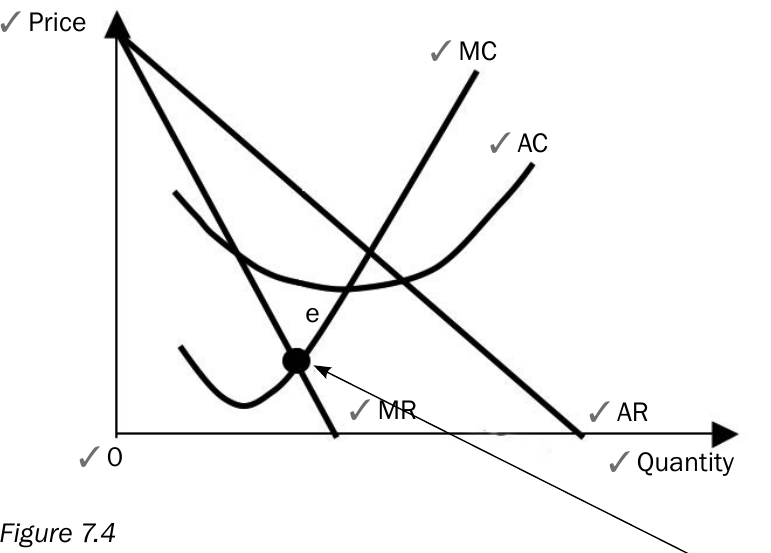
Step 2: Adding revenue curves Draw the two revenue curves starting from the price axis and moving downward to meet the quantity axis. The marginal revenue (MR) curve should be steeper than the average revenue (AR) curve, with both sloping downward from left to right.
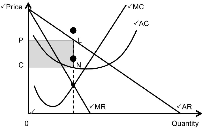
Step 3: Including cost curves Add the marginal cost (MC) and average cost (AC) curves to your diagram. The MC curve typically has a tick-shaped appearance (U-shaped), intersecting the AC curve at its minimum point. This intersection is crucial for understanding cost efficiency.
Step 4: Finding the equilibrium point The most important point on your graph is where MC equals MR. This intersection point (marked as 'e') represents the profit-maximising production level. At this point, the cost of producing one additional unit exactly equals the revenue that unit generates.
Step 5: Determining price and profit From the equilibrium point, draw a vertical line upward to meet the AR curve (demand curve) to find the market price. Draw a horizontal line to meet the AC curve to find the average cost per unit. The rectangular area between these two price levels represents the economic profit earned by the monopolist.
Calculating economic profit
When analysing the profit-maximising diagram, several key relationships become clear:
- The cost structure for monopolists follows the same patterns as competitive businesses
- The profit-maximising output occurs where MC = MR, not where MC = AR (as in perfect competition)
- The market price is determined by moving vertically from the equilibrium point to the demand curve
- Total revenue exceeds short-term total costs, allowing the monopolist to earn economic profits
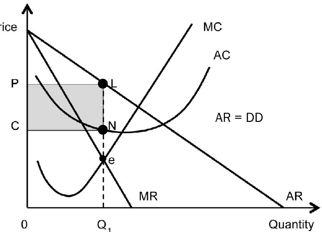
The shaded rectangular area in the diagram represents economic profit, calculated as:
At the profit-maximising output level.
Economic loss in the short term
Not all monopolists automatically earn profits. When market conditions are unfavourable, even monopolists can operate at a loss in the short term.
Conditions for economic loss
Economic losses occur when the average cost curve lies above the demand curve at the profit-maximising output level. In this situation, the cost of production per unit exceeds the price customers are willing to pay, resulting in losses despite the monopolist's market power.
The key difference in the loss scenario is that the AC curve shifts upward and to the right, completely missing intersection with the AR (demand) curve. This indicates that at every possible output level, average costs exceed the maximum price consumers will pay.
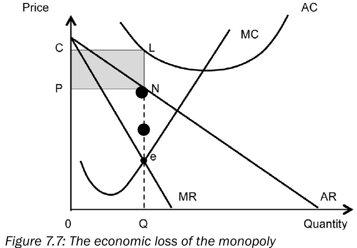
Calculating economic loss
To identify and measure economic loss:
- Find the profit-maximising output where MR = MC
- Determine the market price by extending vertically to meet the AR curve
- Find the average cost by extending horizontally to meet the AC curve
- The loss equals the difference between total cost and total revenue
Economic Loss Calculation:
Understanding loss situations
Three important points about monopolist losses:
- Monopolists suffer short-term losses when the AC curve lies above the demand curve
- Equilibrium still occurs where MR = MC (loss-minimising rather than profit-maximising)
- The monopolist will produce quantity Q and sell at price P, but total costs exceed total revenue
The profitability of any monopolist depends on market demand for their product as well as their production costs, not just their market power.
Comparison between monopoly and perfect markets
Understanding the differences between monopolistic and perfectly competitive markets helps clarify why monopolies behave as they do and what economic effects result from their market power.
| Characteristic | Monopoly | Perfect Market |
|---|---|---|
| Demand curve shape | Downward sloping DD curve, MR curve lies below the DD curve | Horizontal DD curve, MR curve same as DD curve |
| Price determination | Price setter (maker) | Price-taker |
| Market structure | Individual business is the industry | Individual businesses add up to make the industry |
| Consumer response | Consumer buys less if the selling price is high (and vice versa) | Business can't choose its price and if it sells at a different price it loses out |
| Output and efficiency | Monopolist produces lower output at higher prices and in so doing produces at sub-efficient quantities. It does not produce at the minimum point of the LAC curve | Larger output and lower prices. Economically efficient quantities produced. Produces on the lowest point on the AC curve |
| Economic surplus | Producer and consumer surpluses are smaller | Surpluses bigger |
| Product differentiation | Products differentiated - unique - no close substitutes | Product are homogenous |
| Long-term profits | Long-term: can make economic profit | Only normal profit in the long-term |
These differences highlight why economists often view monopolies as less efficient than competitive markets, though monopolies may still serve important economic functions in certain circumstances.
Introduction to oligopolies
Beyond pure monopolies, another important imperfect market structure is the oligopoly, where a small number of large companies control most of the market supply.
Understanding oligopolistic markets
An oligopoly exists when a small number of large companies are able to influence the supply of a product or service to a market. By controlling the supply of the product or service on the market, oligopolies aim to keep prices and profits high.
Real-world examples of oligopolistic industries include oil companies, telecommunications providers, and major retailers. A special type of oligopoly is the duopoly, where only two producers dominate an entire industry.
Key characteristics of oligopolies
Limited competition: Only a few suppliers manufacture the same product, giving each firm significant market influence.
Product variation: Products may be either homogeneous (identical across suppliers) or differentiated (with unique features or branding) that distinguishes one supplier's product from another's.
These characteristics mean that oligopolistic firms must carefully consider their competitors' likely responses when making pricing and output decisions, leading to complex strategic interactions that distinguish oligopolies from both monopolies and perfectly competitive markets.
Key Points to Remember:
- Revenue relationships: For monopolists, the MR curve always lies below the AR (demand) curve, and total revenue follows an inverted U-shape pattern
- Profit maximisation rule: All firms, including monopolists, maximise profits where marginal cost equals marginal revenue (MC = MR)
- Price determination: Monopolists are price setters who determine price by moving from the profit-maximising quantity to the demand curve
- Loss scenarios: Even monopolists can experience economic losses when their average cost curve lies above the market demand curve
- Market efficiency: Monopolies typically produce lower output at higher prices compared to perfectly competitive markets, leading to reduced economic efficiency