Output, Profit, Losses, and Supply (Grade 12 NSC Matric Economics): Revision Notes
Output, Profit, Losses, and Supply
Understanding how firms make production decisions and respond to different profit scenarios is essential for grasping perfect market dynamics. This note explores the relationship between output levels, profitability, and supply decisions that firms face in competitive markets.
Short-term equilibrium positions for individual businesses
In perfect competition, individual firms can find themselves in three possible profit situations depending on how market price compares to their costs. Each scenario leads to different business decisions and market outcomes.
Economic profits
Economic profits occur when a firm's revenue exceeds all its costs, including opportunity costs. This is the most desirable situation for any business owner.
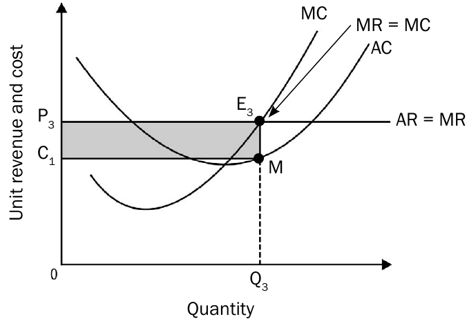
When market price exceeds a firm's average cost, the business earns economic profits. The profit-maximising firm will always produce where marginal revenue equals marginal cost (). In perfect competition, the market price equals both average revenue and marginal revenue ().
In perfect competition, firms are price takers, meaning they accept the market price as given. This is why the demand curve facing an individual firm is perfectly horizontal at the market price level.
The key characteristics of economic profit situations include:
- Market price () is higher than average cost () at the profit-maximising output level
- The firm produces quantity where
- Total revenue exceeds total costs, creating a profit rectangle on the graph
- This profit represents earnings above what the owner could make in the next best alternative
Economic losses
Unfortunately, not all firms enjoy profitable times. Economic losses occur when average costs exceed the market price, meaning the firm cannot cover all its expenses.
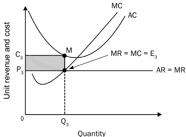
When facing economic losses, firms still follow the profit-maximisation rule of producing where , but now the market price falls below average cost.
Even when making losses, a firm should continue producing in the short run as long as it can cover its variable costs. Shutting down would mean losing all fixed costs, which might result in greater losses than continuing production.
The characteristics of economic loss situations are:
- Market price () is lower than average cost ()
- The firm still produces at where to minimise losses
- Total costs exceed total revenue, creating a loss rectangle
- Whether to continue production depends on comparing price to average variable cost
Normal profits
Normal profit represents the break-even point where total revenue exactly equals total costs, including opportunity costs. This is often called the "zero economic profit" position.
In the normal profit scenario, the market price equals average cost exactly at the profit-maximising output level.
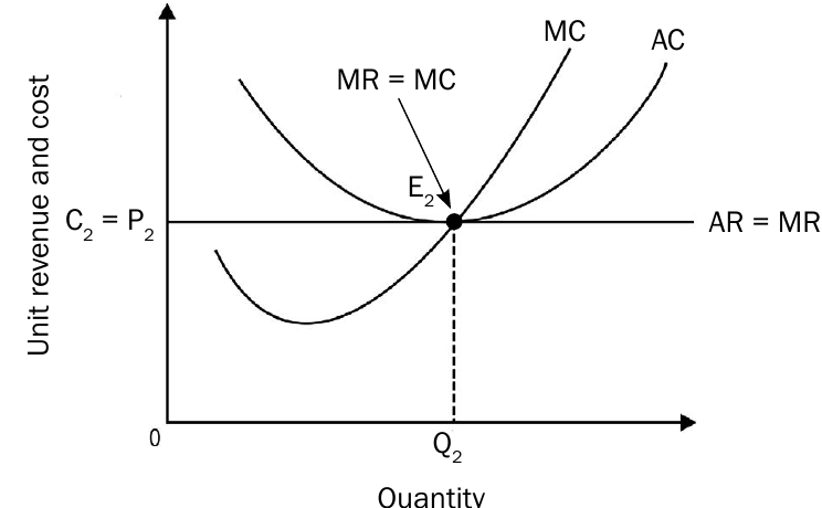
Normal profit characteristics include:
- Market price () equals average cost () at quantity
- The firm covers all costs, including opportunity costs
- No economic profit or loss occurs
- This represents the minimum return needed to keep the owner in the industry
An important distinction exists between short-run and long-run profit expectations. In the short run, firms may experience any of these three profit scenarios. However, in the long run, competitive forces push all firms towards earning normal profits only.
Long-term equilibrium for industry and individual firms
Perfect markets have a remarkable self-correcting mechanism through the entry and exit of firms. This process ensures that long-term equilibrium results in normal profits for all surviving firms.
The impact of entry and exit on equilibrium
Market forces work through firm entry and exit to eliminate economic profits and losses over time. This adjustment process connects individual firm decisions to overall market outcomes.
Entry into profitable markets
When existing firms earn economic profits, this signals attractive opportunities to potential new entrants.
Market Entry Process: The Coffee Shop Example
Imagine a neighbourhood where existing coffee shops are making substantial economic profits due to high demand and limited competition.
Step 1: High profits attract entrepreneurs who notice the opportunity
Step 2: New coffee shops open, increasing the total number of suppliers
Step 3: More coffee shops mean more supply in the market
Step 4: Increased supply leads to lower prices as shops compete
Step 5: Lower prices reduce profits until they return to normal levels
Step 6: Entry stops when profits are no longer above normal
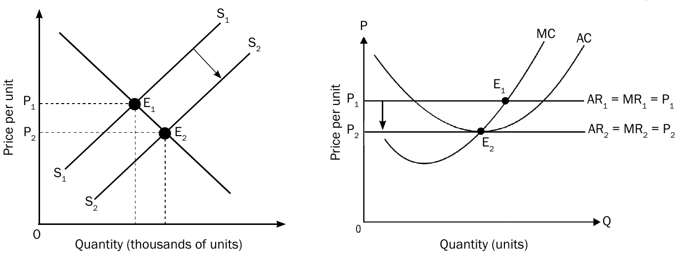
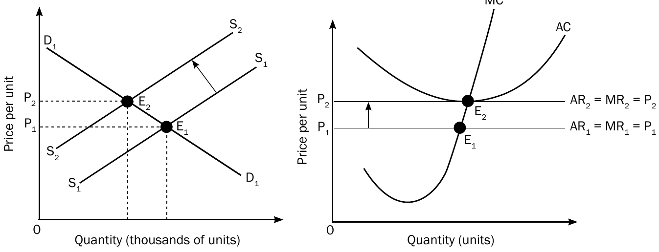
The entry process works as follows:
- Economic profits in the industry attract new firms
- New firms enter the market, increasing total supply
- Market supply curve shifts rightward from to
- Increased supply reduces market price from to
- Individual firms now earn normal profits instead of economic profits
- Entry stops when profits return to normal levels
Exit from unprofitable markets
When firms experience economic losses, some will eventually leave the industry to pursue better opportunities elsewhere.
The exit process operates through:
- Economic losses prompt some firms to leave the industry
- Fewer firms mean reduced market supply
- Supply curve shifts leftward, increasing market price
- Remaining firms return to normal profitability
- Exit stops when losses are eliminated
The entry and exit mechanism is what makes perfect competition so efficient. It automatically eliminates both excess profits and losses, ensuring resources flow to where they're most valued by consumers.
Long-term equilibrium achievement
The entry and exit process continues until all remaining firms earn normal profits. This represents the long-term equilibrium position for perfect markets.
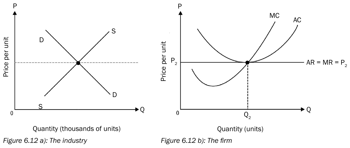
In long-term equilibrium:
- Market price settles at a level where for all firms
- No further entry or exit occurs
- All firms produce at their most efficient scale
- Economic profits and losses are eliminated through market forces
Individual firm's supply curve
Understanding how individual firms decide their production levels helps explain market supply behaviour. The firm's supply curve shows the relationship between market price and the quantity the firm is willing to produce.
Deriving the supply curve
An individual firm's supply curve is actually part of its marginal cost curve, but only above a critical minimum point.
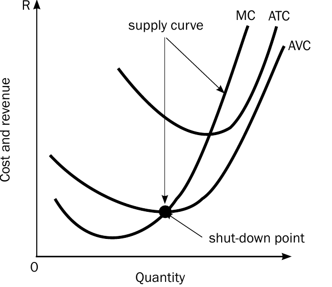
The supply curve is not the entire marginal cost curve. It only includes the portion above the shut-down point, because below this point, the firm would choose to produce nothing rather than operate at a loss greater than its fixed costs.
The supply curve consists of:
- The marginal cost curve above the shut-down point
- No production below the shut-down point
- Increasing quantities supplied as price rises along the MC curve
Shut-down point analysis
The shut-down point represents the critical price level below which a firm should cease production entirely. This occurs when the market price cannot cover the firm's average variable costs.
The Shut-down Rule: A firm should shut down when total revenue is less than total variable costs (), or equivalently, when average revenue falls below average variable cost ().
This is because continuing to produce would mean the firm loses more than just its fixed costs - it would also fail to cover the variable costs of production.
A firm should shut down when:
- Total revenue is less than total variable costs ()
- Average revenue falls below average variable cost ()
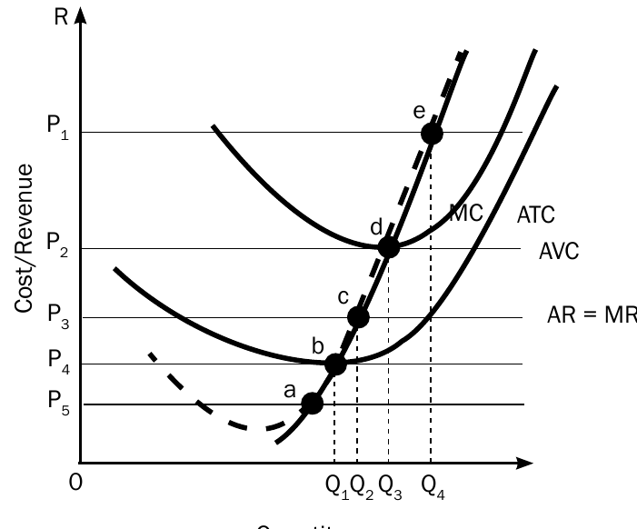
The graph illustrates different price levels and corresponding firm decisions:
- At prices above point e: economic profits
- At point d: normal profits (break-even)
- Between points b and d: economic losses but continue production
- Below point b: shut down production
How to draw equilibrium graphs
Successfully drawing and interpreting equilibrium graphs requires following a systematic approach. These visual tools help analyse firm behaviour under different market conditions.
Step-by-step drawing process
Drawing Perfect Competition Graphs: Step-by-Step Guide
Follow this sequence when constructing equilibrium graphs:
Step 1: Draw the axes
Place Price (P) on the vertical axis and Quantity (Q) on the horizontal axis, ensuring they meet at the origin (0)
Step 2: Add the demand curve
Draw a horizontal demand curve (perfectly elastic in perfect competition), followed by the marginal revenue curve (in perfect competition, D = MR = AR)
Step 3: Draw the AC curve
Add a U-shaped average cost curve showing the typical cost structure
Step 4: Add the MC curve
Draw the marginal cost curve, ensuring it intersects the AC curve at its minimum point
Step 5: Find the profit-maximising point
Identify where MC = MR for optimal production
Step 6: Determine quantity
Drop a vertical line from the profit-maximising point to the x-axis
Step 7: Determine price
The price is given by the market (horizontal demand curve)
Step 8: Analyse profitability
Compare AR/price to AC to determine if the firm makes profits, losses, or normal profits
Remember to label all curves, axes, and important points clearly. Each element serves a specific purpose in economic analysis, so attention to detail matters for accurate interpretation.
Key Points to Remember:
- Profit maximisation rule: All firms maximise profits (or minimise losses) by producing where , regardless of their profit situation
- Three profit scenarios: Economic profits occur when , economic losses when , and normal profits when
- Long-run adjustment: Entry and exit of firms ensure that long-run equilibrium results in normal profits for all surviving firms in perfect competition
- Supply curve derivation: An individual firm's supply curve is the portion of its marginal cost curve above the shut-down point
- Shut-down decision: Firms should cease production when market price falls below average variable cost (), as continuing would increase losses beyond fixed costs