Review of Production, Costs, and Revenue Revision Notes for Grade 12 NSC Matric Economics

Review of Production, Costs, and Revenue

Understanding production, costs, and revenue is essential for analysing how businesses operate and make decisions. These concepts form the foundation for studying market structures and help explain how firms maximise their profits in different economic environments.

Production time periods

Production occurs within different time horizons, and understanding these periods is crucial for analysing business behaviour.

chatImportant

The distinction between short run and long run production is fundamental to understanding how businesses respond to changing market conditions and make strategic decisions.

Short run production refers to a period where only some factors of production can be changed. Specifically, variable factors like labour and raw materials can be adjusted, but fixed factors such as factory size or machinery remain constant. The time period is too brief to allow the number of firms in an industry to change significantly.

Long run production encompasses a period where all factors of production can be modified. This extended timeframe allows businesses to change both variable and fixed factors, such as expanding facilities or purchasing new equipment. It also provides sufficient time for new firms to enter an industry or existing firms to exit completely.

infoNote

Think of short run as "working with what you have" while long run represents "changing everything you need to change." A restaurant can hire more staff quickly (short run) but expanding the dining room takes much longer (long run).

Key production, cost, and revenue concepts

Understanding how economists measure and calculate different aspects of business operations helps us analyse firm behaviour more effectively.

Production measurements

These concepts help businesses understand their productivity and efficiency:

Concept	Definition	Formula
Total Product/Output	The maximum output a firm can produce using all available fixed and variable inputs	-
Marginal Product/Output	The additional output produced when one more unit of variable input (typically labour) is combined with fixed inputs	$MP = \frac{\Delta TP}{\Delta Q}$
Average Product/Output	The contribution each unit of variable input makes towards total production	$AP = \frac{P}{Q}$

Cost classifications

Understanding different types of costs is essential for business decision-making:

Concept	Definition	Formula
Fixed Costs	Expenses that remain constant regardless of output levels (e.g., rent, insurance, depreciation)	-
Variable Costs	Expenses that change with production levels (e.g., wages, raw materials, electricity)	-
Total Cost	The complete cost of all factors used in production	$TC = FC + VC$
Marginal Cost	The additional cost incurred when producing one extra unit of output	$MC = \frac{\Delta TC}{\Delta Q}$
Average Cost	The cost per unit of production	$AC = AFC + AVC$ or $\frac{TC}{Q}$
Average Fixed Cost	Fixed costs divided by the quantity produced	$AFC = \frac{FC}{Q}$
Average Variable Cost	Variable costs divided by the quantity produced	$AVC = \frac{VC}{Q}$

Revenue measurements

These measurements help businesses understand their income patterns:

Concept	Definition	Formula
Total Revenue	The complete income received from selling goods or services	$TR = P \times Q$
Marginal Revenue	The extra income earned from selling one additional unit	$MR = \frac{\Delta TR}{\Delta Q}$
Average Revenue	The income earned per unit sold	$AR = \frac{TR}{Q}$

infoNote

Notice how marginal calculations always use the "change in" concept ( $\Delta$ ), while average calculations divide totals by quantity. This pattern makes the formulas easier to remember!

Practical cost analysis: Kael's pie shop

lightbulbExample

Worked Example: Cost Analysis for a Small Business

Let's examine how these concepts work in practice using data from Kael's pie shop:

Quantity (Q)	Total Fixed Costs (TFC)	Total Variable Costs (TVC)	Total Costs	Average Fixed Cost (AFC)	Average Variable Cost (AVC)	Average Total Cost (ATC)	Marginal Cost (MC)
0	120	0	120	-	-	-	-
10	120	100	220	12	10	22	10
20	120	160	280	6	8	14	6
30	120	210	330	4	7	11	5
40	120	280	400	3	7	10	7
50	120	400	520	2.4	8	10.4	12
60	120	600	720	2	10	12	20
70	120	910	1030	1.7	13	14.7	31

Key observations from this data:

Fixed costs remain constant at R120 regardless of production level
Variable costs increase as production rises, but not always at the same rate
Average fixed costs decrease continuously as output increases because the same fixed cost is spread over more units
Marginal costs initially decrease then increase, creating a U-shaped pattern

Understanding cost curve relationships

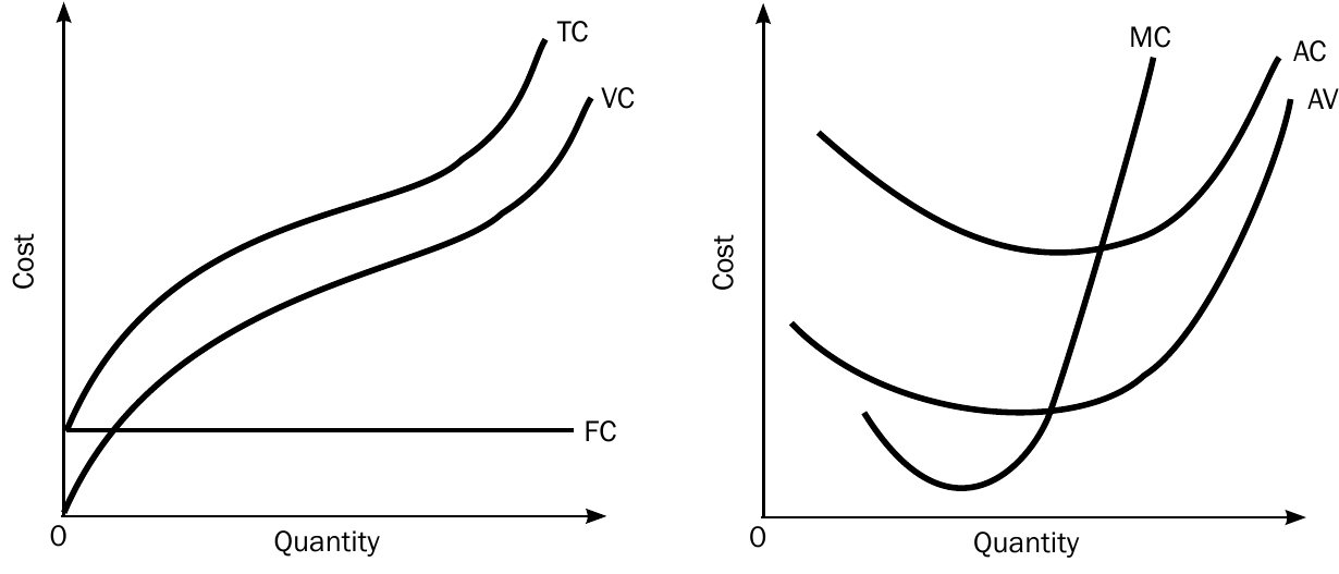
The graphical representation of costs helps visualise important economic relationships. The left graph shows how total costs behave, while the right graph illustrates per-unit cost patterns.

Important cost curve observations

Several key principles govern how cost curves interact, and understanding these relationships is crucial for business analysis:

chatImportant

Critical Cost Curve Relationships:

The following relationships are fundamental to understanding business cost behaviour:

The gap between total cost and variable cost curves equals fixed costs. Since $TC = FC + VC$ , the vertical distance between these curves always represents the constant fixed costs.
Variable cost curves start from zero, while total cost curves begin at the fixed cost level. When production is zero, there are no variable costs, but fixed costs still exist.
The gap between average cost and average variable cost decreases as output increases. This happens because average fixed costs (the difference between AC and AVC) fall as production rises.
Marginal cost curves intersect both average cost and average variable cost curves at their minimum points. This is a fundamental economic principle: when marginal cost is below average cost, it pulls the average down; when marginal cost is above average cost, it pushes the average up.

These relationships help businesses understand how their costs will behave as they change production levels, enabling better planning and decision-making.

infoNote

The intersection of marginal cost with average cost curves at their minimum points is similar to how your marginal test score affects your overall average - if your latest score is below your average, it pulls the average down!

bookmarkSummary

Key Points to Remember:

Short run vs long run: In the short run, only variable factors can change; in the long run, all factors can be adjusted
Total cost relationship: $TC = FC + VC$ - This fundamental relationship helps separate costs that change with production from those that don't
Marginal measurements: Show the change from producing one more unit - These calculations are crucial for deciding whether to increase or decrease production
Average fixed costs: Always decrease as production increases - Fixed costs spread over more units means lower per-unit fixed costs
Cost curve intersection: Marginal cost curves cut average cost curves at their lowest points - This relationship helps identify the most efficient production level

Review of Production, Costs, and Revenue (Grade 12 NSC Matric Economics): Revision Notes