Applications of Differential Calculus Revision Notes for Grade 12 NSC Matric Mathematics

Applications of Differential Calculus

Optimisation problems

Optimisation problems are mathematical problems where we need to find the maximum or minimum value of a quantity. These problems appear frequently in real-world situations such as maximising profits, minimising costs, or finding the most efficient solutions.

Differential calculus provides us with powerful tools to solve these problems by finding stationary points - points where the rate of change is zero.

Finding the optimum point

To solve optimisation problems, follow this systematic approach:

Set up the problem - Define variables and write equations
Express the quantity to optimize - Write as a function of one variable only
Find the derivative and set it equal to zero: $f'(x) = 0$
Solve for the critical values
Use the second derivative test to determine if it's a maximum or minimum
Write the final answer in context

chatImportant

The quantity to be optimised must be expressed in terms of only one variable before you can differentiate and find the optimum point.

Second derivative test

Once you find the stationary points by setting $f'(x) = 0$ , use the second derivative to classify them:

If $f''(a) < 0$ , then $x = a$ gives a local maximum
If $f''(a) > 0$ , then $x = a$ gives a local minimum

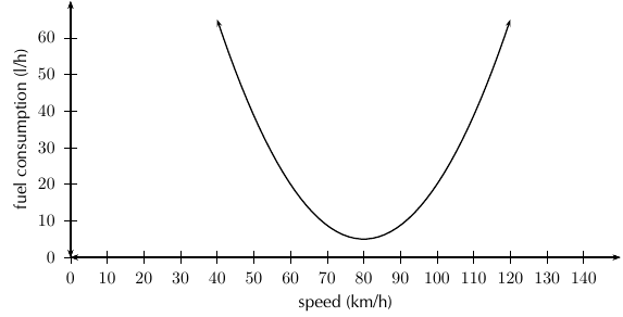
The fuel consumption graph above shows a classic optimisation problem where there is an optimal speed that minimises fuel usage.

lightbulbExample

Worked Example 1: Maximising a Product

Question: The sum of two positive numbers is 10. One number is multiplied by the square of the other. Find the numbers that make this product maximum.

Solution:

Step 1: Set up the equations Let the two numbers be $a$ and $b$ , with product $P$ .

$a + b = 10$ ... (1)
$P = a \times b^2$ ... (2)

Step 2: Express in terms of one variable

From equation (1): $b = 10 - a$

Substitute into equation (2): $P = a(10 - a)^2$

Expanding: $P(a) = a(100 - 20a + a^2) = 100a - 20a^2 + a^3$

Step 3: Find the derivative $P'(a) = 100 - 40a + 3a^2$

Step 4: Find stationary points

Set $P'(a) = 0$ :

$100 - 40a + 3a^2 = 0$

$3a^2 - 40a + 100 = 0$

Using factorisation: $(3a - 10)(a - 10) = 0$

Therefore: $a = \frac{10}{3}$ or $a = 10$

Step 5: Check which gives maximum using second derivative

$P''(a) = 6a - 40$

For $a = \frac{10}{3}$ : $P''\left(\frac{10}{3}\right) = 6\left(\frac{10}{3}\right) - 40 = 20 - 40 = -20 < 0$

This confirms $a = \frac{10}{3}$ gives a maximum.

Step 6: Find the corresponding value of b

When $a = \frac{10}{3}$ : $b = 10 - \frac{10}{3} = \frac{20}{3}$

Answer: The two numbers are $\frac{10}{3}$ and $\frac{20}{3}$ that give the maximum product.

lightbulbExample

Worked Example 2: Garden Fencing Optimization

Question: Michael wants to fence a rectangular vegetable garden using a wall as one border. He has 160 m of fencing. Calculate the dimensions that give the largest possible area.

Solution:

Step 1: Set up the problem Let width = $w$ and length = $l$

Area = $w \times l$
Fencing needed: $w + l + l = 160$ (since wall provides one side)
Therefore: $w + 2l = 160$

Step 2: Express area in terms of one variable

From the constraint: $w = 160 - 2l$

Area = $l(160 - 2l) = 160l - 2l^2$

Step 3: Find the derivative

$\frac{dA}{dl} = 160 - 4l$

Step 4: Find stationary point

Set $\frac{dA}{dl} = 0$ :

$160 - 4l = 0$

$4l = 160$

$l = 40$

Step 5: Check it's a maximum

$\frac{d^2A}{dl^2} = -4 < 0$ , confirming maximum

Step 6: Calculate width

$w = 160 - 2(40) = 160 - 80 = 80$

Answer: The garden should be 80 m wide and 40 m long for maximum area.

infoNote

Important Optimisation Tips:

Always check your answer makes practical sense in the real-world context
Consider the domain restrictions (e.g., dimensions must be positive)
Use the second derivative test to confirm whether you have a maximum or minimum

Rates of change

Rate of change describes how fast one quantity changes with respect to another. In mathematics, we can represent these changes using derivatives.

Understanding rates of change is fundamental in many real-world applications, from analysing motion to studying economic trends and population growth.

Average vs instantaneous rates of change

Average rate of change = $\frac{f(x + h) - f(x)}{(x + h) - x} = \frac{f(x + h) - f(x)}{h}$

Instantaneous rate of change = $\lim_{h \to 0} \frac{f(x + h) - f(x)}{h} = f'(x)$

infoNote

When we simply mention "rate of change," we typically mean the instantaneous rate of change (the derivative).

Velocity and acceleration

Velocity is one of the most common applications of rates of change:

Average velocity = Average rate of change of distance
Instantaneous velocity = Instantaneous rate of change of distance = Derivative

If $s(t)$ represents distance at time $t$ , then:

Velocity: $v(t) = \frac{ds}{dt} = s'(t)$
Acceleration: $a(t) = \frac{dv}{dt} = v'(t) = s''(t)$

chatImportant

Acceleration is the rate of change of velocity, which means it's the second derivative of distance. This relationship is crucial for understanding motion problems.

lightbulbExample

Worked Example 3: Golf Ball Motion Analysis

Question: The height (in metres) of a golf ball $t$ seconds after being hit is given by $H(t) = 20t - 5t^2$ . Find:

The average velocity during the first two seconds
The velocity after 1.5 s
The time when velocity is zero
The velocity when hitting the ground
The acceleration

Solution:

Step 1: Average velocity in first two seconds

Average velocity = $\frac{H(2) - H(0)}{2 - 0}$

= $\frac{[20(2) - 5(2)^2] - [20(0) - 5(0)^2]}{2}$
= $\frac{40 - 20 - 0}{2} = \frac{20}{2} = 10{m·s}^{-1}$

Step 2: Instantaneous velocity

$v(t) = H'(t) = \frac{dH}{dt} = 20 - 10t$

Velocity after 1.5 s: $v(1.5) = 20 - 10(1.5) = 20 - 15 = 5 {m·s}^{-1}$

Step 3: Time when velocity is zero

Set $v(t) = 0$ :

$20 - 10t = 0$
$10t = 20$
$t = 2$

The velocity is zero after 2 seconds.

Step 4: Velocity when hitting ground

Ball hits ground when $H(t) = 0$ :

$20t - 5t^2 = 0$
$5t(4 - t) = 0$
$t = 0$ or $t = 4$

The ball hits the ground after 4 seconds.

Velocity at $t = 4$ : $v(4) = 20 - 10(4) = 20 - 40 = -20 {m·s}^{-1}$

The negative sign indicates downward motion.

Step 5: Acceleration

$a(t) = v'(t) = H''(t) = -10$

The acceleration is constant at $-10 {m·s}^{-2}$ (due to gravity).

Key formulas for rates of change

Average rate of change = $\frac{\Delta y}{\Delta x} = \frac{\text{change in output}}{\text{change in input}}$
Instantaneous rate of change = $\frac{dy}{dx} = f'(x)$
Velocity = $\frac{ds}{dt}$ where $s$ = distance, $t$ = time
Acceleration = $\frac{dv}{dt} = \frac{d^2s}{dt^2}$ where $v$ = velocity

bookmarkSummary

Key Points to Remember:

Set $f'(x) = 0$ to find stationary points for optimisation problems
Use the second derivative test to determine maximum $(f'' < 0)$ or minimum $(f'' > 0)$
Express optimisation problems in terms of one variable only before differentiating
Rate of change problems often involve velocity (first derivative) and acceleration (second derivative)
Always check your answers make practical sense in the context of the problem

Applications of Differential Calculus (Grade 12 NSC Matric Mathematics): Revision Notes