The Reciprocal Transformation Revision Notes for VCE SSCE General Mathematics

The Reciprocal Transformation

What is a reciprocal transformation?

A reciprocal transformation is a type of stretching transformation used to linearise non-linear data. It works by compressing the upper end of the scale on either the $x$ -axis or $y$ -axis. This compression is more dramatic than what you get with a logarithmic transformation.

The reciprocal transformation takes a variable and transforms it by calculating its reciprocal (one divided by the variable). For example:

If you have a variable $x$ , the reciprocal transformation gives you $\frac{1}{x}$
If you have a variable $y$ , the reciprocal transformation gives you $\frac{1}{y}$

When to use reciprocal transformations

infoNote

Use reciprocal transformations when you have a curved relationship between two variables that needs to be straightened out so you can fit a linear regression line. You can apply the transformation to either the explanatory variable ( $x$ ) or the response variable ( $y$ ), depending on the shape of your data.

How reciprocal transformations work

The $\frac{1}{x}$ transformation

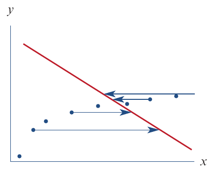
When you apply a reciprocal transformation to the explanatory variable (the $x$ -axis):

Effect on scale: The transformation compresses larger $x$ values relative to smaller values. This compression is stronger than what you'd get with a logarithmic transformation.
Straightening curves: This transformation is particularly good at straightening out certain types of curved patterns in scatterplots.
Data reversal: An important property to remember is that the transformation reverses the order of your data values. Values of $x$ that were less than 1 become greater than 1, and values that were greater than 1 become less than 1. Think of it as flipping the data around the value of 1.

The $\frac{1}{y}$ transformation

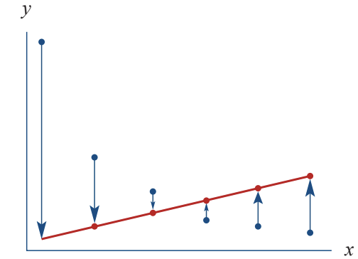
When you apply a reciprocal transformation to the response variable (the $y$ -axis):

Effect on scale: The transformation compresses larger $y$ values relative to smaller values.
Straightening curves: This transformation straightens out different types of curved patterns compared to the $\frac{1}{x}$ transformation.
Data reversal: Just like with $\frac{1}{x}$ , the order of the data values is reversed around the value of 1.

chatImportant

Remember the Reversal Property

Both $\frac{1}{x}$ and $\frac{1}{y}$ transformations reverse the order of data values around 1. This means:

Values less than 1 become greater than 1
Values greater than 1 become less than 1

This reversal property is crucial for understanding how the transformation affects your data!

Worked example: Applying the $\frac{1}{x}$ transformation

Let's look at a real-world example to understand how the $\frac{1}{x}$ transformation works.

Context: Ben started a healthy eating and exercise plan and recorded his weekly weight loss over 10 weeks. When we plot this data, we see a curved relationship between the length of the diet and weekly weight loss.

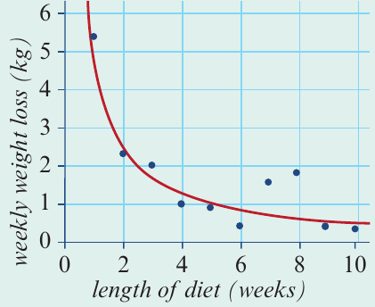
The scatterplot shows a strong negative association, but it's clearly not linear. As the diet continues for more weeks, the weekly weight loss decreases, but the relationship is curved.

lightbulbExample

Worked Example: Linearising Diet Data

Step 1: Apply the reciprocal transformation

To linearise this data, we transform the explanatory variable (length of diet) by calculating $\frac{1}{\text{length of diet}}$ for each data point.

After applying this transformation, the new scatterplot plots weekly weight loss against $\frac{1}{\text{length of diet}}$ :

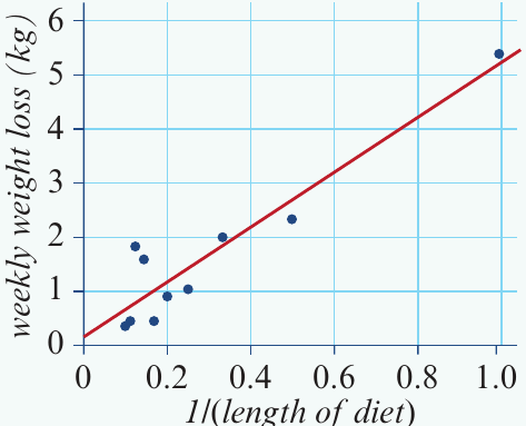
Notice how the data points now form a much straighter pattern! The transformation has successfully linearised the relationship.

Step 2: Fit a least squares regression line

Now that the data is linear, we can fit a least squares regression line. For this example, the equation is:

$\text{weekly weight loss} = 0.13 + \frac{5.09}{\text{length of diet}}$

Step 3: Make predictions

We can use this equation to make predictions. For example, to predict the weight loss in week 11:

\begin{aligned} \text{weekly weight loss} &= 0.13 + \frac{5.09}{11} \\ &= 0.13 + 0.46 \\ &= 0.6 \text{ kg} \end{aligned}

Notice how we substitute the original value (week 11) directly into the equation, not its reciprocal.

Worked example: Applying the $\frac{1}{y}$ transformation

Now let's see how the $\frac{1}{y}$ transformation works with a different example.

Context: A homeware company makes rectangular sticky labels with various lengths and widths. The table below shows the dimensions of eight different labels:

Length (cm)	6.8	5.6	4.6	4.2	3.5	4.0	5.0	5.5
Width (cm)	1.8	2.0	2.5	3.0	3.5	2.6	2.0	1.9

When we plot width against length, we see a curved relationship:

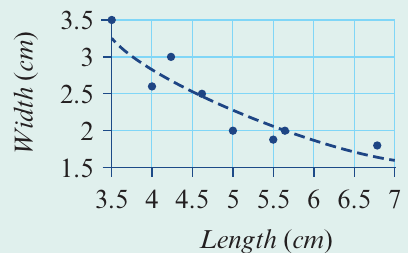
There's a strong negative association, but it's clearly non-linear.

lightbulbExample

Worked Example: Linearising Sticky Label Data

Step 1: Apply the reciprocal transformation

This time, we transform the response variable (width) by calculating $\frac{1}{\text{width}}$ for each data point.

After applying this transformation, we plot $\frac{1}{\text{width}}$ against length:

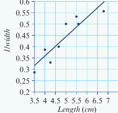
The relationship is now linear!

Step 2: Fit a least squares regression line

The equation of the least squares line fitted to the transformed data is:

$\frac{1}{\text{width}} = 0.015 + 0.086 \times \text{length}$

Step 3: Make predictions

To predict the width of a sticky label that is 5 cm long:

First, substitute into the equation:

\begin{aligned} \frac{1}{\text{width}} &= 0.015 + 0.086 \times 5 \\ \frac{1}{\text{width}} &= 0.015 + 0.430 \\ \frac{1}{\text{width}} &= 0.445 \end{aligned}

Then, to find the actual width, take the reciprocal of both sides:

\begin{aligned} \text{width} &= \frac{1}{0.445} \\ \text{width} &= 2.25 \text{ cm} \end{aligned}

chatImportant

Critical Step: Back-Transformation Required!

When you transform the response variable ( $y$ ), you must back-transform your prediction to get the answer in the original units. This means taking the reciprocal of your calculated value.

Forgetting this step is a common mistake that will cost you marks in exams!

Key differences between $\frac{1}{x}$ and $\frac{1}{y}$ transformations

Understanding which transformation to use is important:

infoNote

Use $\frac{1}{x}$ transformation when:

The curve in your scatterplot bends in a particular way where larger $x$ values need to be compressed
You can substitute directly into the equation without back-transformation

Use $\frac{1}{y}$ transformation when:

The curve in your scatterplot requires compression of larger $y$ values
You need to remember to back-transform (take the reciprocal) of your final answer

Exam tips

infoNote

Essential Exam Tips

Check the shape of the curve: Look carefully at your scatterplot to decide whether you need to transform $x$ or $y$ .
Remember the back-transformation: If you transform $y$ , you must take the reciprocal of your calculated value to get the final answer in the original units.
Show your working: Always write out each step clearly, especially when back-transforming.
Use correct units: Make sure your final answer has the appropriate units from the original data.
Understand the reversal effect: Remember that reciprocal transformations reverse the order of data values around 1. This can help you check if your transformation makes sense.

Summary

bookmarkSummary

Key Points to Remember:

Reciprocal transformations compress the upper end of the scale on either the $x$ -axis or $y$ -axis, providing stronger compression than logarithmic transformations.
The $\frac{1}{x}$ transformation compresses larger $x$ values and reverses the data order. You can use the transformed equation directly for predictions.
The $\frac{1}{y}$ transformation compresses larger $y$ values and reverses the data order. You must back-transform predictions by taking the reciprocal to get the final answer.
Both transformations are used to linearise curved data so that a least squares regression line can be fitted and used for predictions.
Always check your scatterplot after transformation to ensure the relationship has become linear before fitting a regression line.

The Reciprocal Transformation (VCE SSCE General Mathematics): Revision Notes