Fitting a Least Squares Regression Line to Numerical Data Revision Notes for VCE SSCE General Mathematics

Fitting a Least Squares Regression Line to Numerical Data

What is linear regression?

When we want to model the relationship between two numerical variables with a straight line, we use a process called linear regression. The line we create is known as the regression line.

Every straight line can be described using an equation in the form:

$y = a + bx$

In this equation:

$a$ represents the y-intercept (where the line crosses the y-axis)
$b$ represents the slope (how steep the line is)

To fit a line to our data, we need to find the best values for $a$ and $b$ that make the line pass as close as possible to all our data points.

Methods for fitting a line

There are two main approaches to fitting a line to bivariate data:

Drawing by eye

The simplest method is to plot your data on a scatterplot and draw a line with a ruler that seems to follow the general pattern. However, this method has a major weakness: different people will draw different lines, making it unreliable and inconsistent.

The least squares method

The more rigorous approach is the least squares method. This mathematical technique finds the one line that best fits the data according to a specific criterion. The method assumes the variables have a linear relationship and works most effectively when there are no obvious outliers in your data.

Understanding residuals

Before we can explain the least squares method, we need to understand what a residual is.

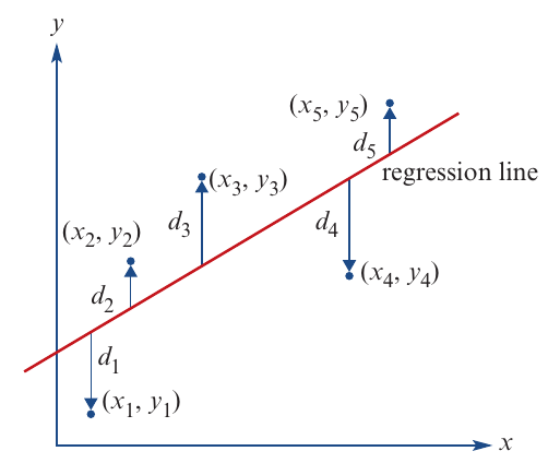
A residual is the vertical distance between an actual data point and the regression line. In other words, it measures how far each point is from the line.

Residuals can be:

Positive: when the data point sits above the regression line
Negative: when the data point sits below the regression line
Zero: when the data point falls exactly on the regression line

infoNote

Think of residuals as prediction errors. If we use the regression line to predict a value and the actual value is different, the residual tells us how much our prediction was off by.

The least squares line

The least squares line is special because it minimises the sum of the squares of all the residuals. Mathematically, this means it makes this expression as small as possible:

$d_1^2 + d_2^2 + d_3^2 + d_4^2 + d_5^2$

where $d_1, d_2, d_3$ , etc. are the residuals.

Why do we square the residuals?

You might wonder why we square the residuals instead of just adding them up. Here's why: if we simply added up all the residuals (without squaring), they would always sum to zero! This happens because the least squares line balances the data, similar to how a see-saw balances weight on both sides. Some residuals are positive and some are negative, and they cancel each other out.

infoNote

Squaring the residuals solves this problem by making all values positive, so we can genuinely minimise the total distance of points from the line.

Assumptions for using the least squares method

Before fitting a least squares line, we must check that our data meets three important conditions:

chatImportant

Critical Assumptions for Least Squares Regression:

The data must be numerical - both variables need to be measured on a numerical scale
The association must be linear - the relationship between variables should form a roughly straight pattern
There should be no clear outliers - extreme values can distort the regression line

These are the same assumptions we use when calculating the correlation coefficient.

Formulas for the least squares regression line

To find the equation of the least squares line, we need to calculate the slope ( $b$ ) and intercept ( $a$ ). While the mathematics behind these formulas involves calculus, you can use these rules:

Slope:

$b = \frac{rs_y}{s_x}$

Intercept:

$a = \bar{y} - b\bar{x}$

Where:

$r$ is the correlation coefficient
$s_x$ and $s_y$ are the standard deviations of $x$ and $y$
$\bar{x}$ and $\bar{y}$ are the mean values of $x$ and $y$
$y$ is the response variable (what we want to predict)
$x$ is the explanatory variable (what we use to make predictions)

Finding the correlation coefficient from the slope

If you know the slope of the regression line but need to find the correlation coefficient, you can rearrange the slope formula:

$r = \frac{bs_x}{s_y}$

chatImportant

Critical: Always Calculate Slope First!

You must correctly identify which variable is explanatory ( $x$ ) and which is response ( $y$ ) before you start your calculations. Getting this wrong will give you an incorrect regression line. The question will usually tell you which variable predicts which (for example, "predict weight from height" means height is the explanatory variable).

Worked example 1: Finding the regression line using summary statistics

lightbulbExample

Worked Example: Calculating the Least Squares Regression Line

Question: The height and weight of 11 people have been recorded. The following statistics were calculated:

Table

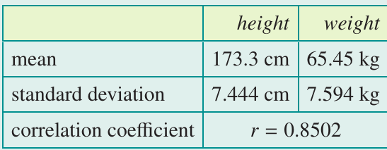
Use the formulas to find the equation of the least squares regression line that enables weight to be predicted from height. Round the slope and intercept to two decimal places.

Solution:

Step 1: Identify the variables

Since we want to predict weight from height:

Explanatory variable (EV): height ( $x$ )
Response variable (RV): weight ( $y$ )

Step 2: Write down the given information

$\bar{x} = 173.3, \quad s_x = 7.444$

$\bar{y} = 65.45, \quad s_y = 7.594$

$r = 0.8502$

Step 3: Calculate the slope

$b = \frac{rs_y}{s_x}$

$b = \frac{0.8502 \times 7.594}{7.444}$

$b = 0.87$ (rounded to two decimal places)

Step 4: Calculate the intercept

$a = \bar{y} - b\bar{x}$

$a = 65.45 - 0.87 \times 173.3$

$a = -84.86$ (rounded to two decimal places)

Step 5: Write the regression equation

Using the calculated values:

$y = -84.86 + 0.87x$

Or in terms of the actual variables:

$\text{weight} = -84.86 + 0.87 \times \text{height}$

Worked example 2: Finding the correlation coefficient from the slope

lightbulbExample

Worked Example: Finding the Correlation Coefficient

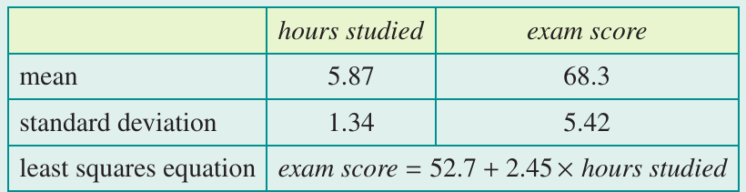
Question: Use the following information to find the correlation coefficient $r$ , rounded to three decimal places.

Table

Solution:

Step 1: Identify the variables

Explanatory variable (EV): hours studied ( $x$ )
Response variable (RV): exam score ( $y$ )

Step 2: Write down the given information

From the least squares equation, we can see that $b = 2.45$

$s_x = 1.34, \quad s_y = 5.42$

Step 3: Calculate the correlation coefficient

Using the rearranged formula:

$r = \frac{bs_x}{s_y}$

$r = \frac{2.45 \times 1.34}{5.42}$

$r = 0.606$ (rounded to three decimal places)

Using technology to find the regression line

Modern calculators like the TI-Nspire CAS and ClassPad can calculate the least squares regression line automatically. This is much faster than using formulas by hand, especially with large datasets.

Basic process using a calculator

Here's the general approach:

Enter your data into two lists or columns (one for each variable)
Create a scatterplot to visualise the relationship
Identify which variable is explanatory and which is response
Use the regression function to calculate the line equation
Display the regression line on your scatterplot

infoNote

The calculator will provide:

The equation of the regression line
The slope ( $b$ ) and intercept ( $a$ )
The coefficient of determination ( $r^2$ )

This saves significant time and reduces calculation errors, especially when working with large datasets.

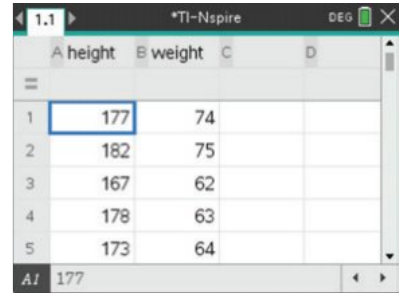
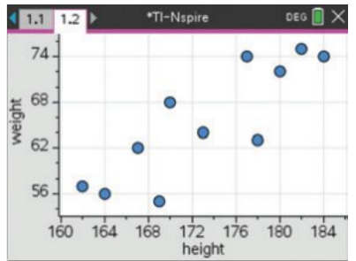
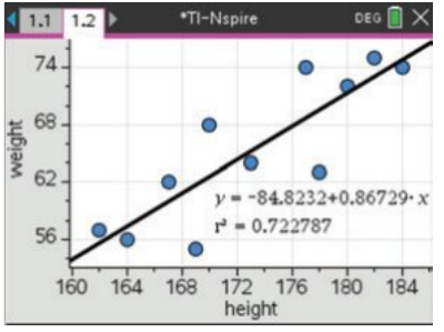
For example, with the height and weight data, the calculator produces:

$\text{weight} = -84.8 + 0.867 \times \text{height}$

with $r^2 = 0.723$

This matches our manual calculation from Example 1.

Exam tips

infoNote

Essential Tips for Success:

Always start by identifying which variable is explanatory and which is response
Calculate the slope first, then use it to find the intercept
Round your final answers appropriately (check what the question asks for)
Check that your regression line makes sense by looking at the scatterplot
Remember: correlation doesn't equal causation, even with a strong regression line
Write your final equation using the actual variable names, not just $x$ and $y$

Key takeaways

bookmarkSummary

Key Points to Remember:

Linear regression models the relationship between two numerical variables using a straight line
Residuals are the vertical distances from data points to the regression line
The least squares line minimises the sum of squared residuals, making it the best-fitting line
Calculate slope using: $b = \frac{rs_y}{s_x}$
Calculate intercept using: $a = \bar{y} - b\bar{x}$
Always identify the explanatory variable ( $x$ ) and response variable ( $y$ ) before calculating
The method assumes numerical data, linear association, and no clear outliers

Fitting a Least Squares Regression Line to Numerical Data (VCE SSCE General Mathematics): Revision Notes