Data Transformations Revision Notes for VCE SSCE General Mathematics

Data Transformations

Introduction to data transformations

When we plot data from two variables on a graph, we might notice a clear relationship between them that is not linear (not a straight line). To make these relationships easier to analyse, we can transform the data by changing the scale of one variable using a mathematical function.

infoNote

Transforming the data means changing the scale of a variable by applying a mathematical function to its values.

Linearisation is the process of transforming data so that a non-linear relationship becomes linear (a straight line). This makes the relationship much easier to analyse using methods we already know.

In this section, we focus on two important transformations:

The squared transformation ( $x^2$ )
The reciprocal transformation ( $\frac{1}{x}$ )

The squared transformation: $x^2$

What is the squared transformation?

In the squared transformation, we change the scale on the horizontal axis from $x$ to $x^2$ . This means instead of plotting our data points using the original $x$ values, we square each $x$ value first and then plot $y$ against $x^2$ .

When do we use it?

infoNote

The squared transformation is useful when we have a parabolic (curved) relationship between variables. This type of relationship often appears in situations involving direct variation with a power, such as $y \propto x^2$ .

Example from physics

lightbulbExample

Worked Example: Distance and Time for a Falling Object

Consider a metal ball dropped from a tall building. The distance fallen ( $d$ ) and time ( $t$ ) have a relationship where $d = 4.91t^2$ .

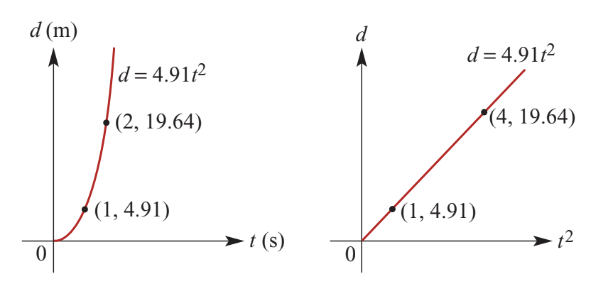
On the left, the graph of $d$ against $t$ is curved (a parabola). However, when we plot $d$ against $t^2$ (on the right), we get a straight line through the origin. The slope of this line equals the constant of variation (4.91 in this case).

How to perform the squared transformation

Step 1: Start with your table of $x$ and $y$ values

$x$	0	1	2	3	4
$y$	1	2	5	10	17

Step 2: Plot the original data ( $y$ against $x$ )

This will typically show a curved relationship.

Step 3: Create a new row by squaring all $x$ values

$x$	0	1	2	3	4
$x^2$	0	1	4	9	16
$y$	1	2	5	10	17

Step 4: Plot the transformed data ( $y$ against $x^2$ )

chatImportant

Make sure to label the horizontal axis as $x^2$ , not $x$ .

Step 5: Check if the graph is linear

If the points form a straight line, the transformation has successfully linearised the data. The slope of this line is the constant of variation.

bookmarkSummary

Key Points About the Squared Transformation:

If $y \propto x^2$ , then plotting $y$ against $x^2$ produces a straight line through the origin
The slope of the resulting line equals the constant of variation ( $k$ )
This transformation is particularly useful for quadratic relationships

The reciprocal transformation: $\frac{1}{x}$

What is the reciprocal transformation?

In the reciprocal transformation, we change the scale on the horizontal axis from $x$ to $\frac{1}{x}$ . This means we calculate the reciprocal (one divided by each value) of each $x$ value and plot $y$ against $\frac{1}{x}$ .

When do we use it?

infoNote

The reciprocal transformation is useful when we have a hyperbolic relationship between variables. This type of relationship appears in situations involving inverse variation, such as $y \propto \frac{1}{x}$ .

Example of inverse variation

Consider the relationship $y = \frac{6}{x}$ , where the constant of variation is 6.

The table shows both $x$ values and their reciprocals $\frac{1}{x}$ :

$x$	$\frac{1}{3}$	$\frac{1}{2}$	1	2
$\frac{1}{x}$	3	2	1	$\frac{1}{2}$
$y$	18	12	6	3

When we plot $y$ against $x$ , we get a curved line (hyperbola). However, when we plot $y$ against $\frac{1}{x}$ , we get a straight line with slope 6.

chatImportant

The graph will not have a point at the origin because $\frac{1}{0}$ is undefined.

How to perform the reciprocal transformation

Step 1: Start with your table of $x$ and $y$ values

$x$	1	2	4	5
$y$	10	5	2.5	2

Step 2: Plot the original data ( $y$ against $x$ )

This will typically show a hyperbolic (curved) relationship.

Step 3: Calculate the reciprocal of each $x$ value

lightbulbExample

Worked Example: Calculating Reciprocals

To find $\frac{1}{x}$ , divide 1 by each $x$ value:

$\frac{1}{1} = 1$
$\frac{1}{2} = 0.5$
$\frac{1}{4} = 0.25$
$\frac{1}{5} = 0.2$

$x$	1	2	4	5
$\frac{1}{x}$	1	0.5	0.25	0.2
$y$	10	5	2.5	2

Step 4: Plot the transformed data ( $y$ against $\frac{1}{x}$ )

chatImportant

Remember to label the horizontal axis as $\frac{1}{x}$ , not $x$ .

Step 5: Check if the graph is linear

If the points form a straight line, the transformation has successfully linearised the data. The slope of this line is the constant of variation.

bookmarkSummary

Key Points About the Reciprocal Transformation:

If $y \propto \frac{1}{x}$ , then plotting $y$ against $\frac{1}{x}$ produces a straight line
The line will not pass through the origin because $\frac{1}{0}$ is undefined
The slope of the resulting line equals the constant of variation ( $k$ )
This transformation is particularly useful for inverse relationships

Using technology for transformations

Both the squared and reciprocal transformations can be performed using a CAS (Computer Algebra System) calculator. The general process involves:

Entering your data into lists named $x$ and $y$
Creating a new column for the transformed variable (either $x^2$ or $\frac{1}{x}$ )
Plotting the original data to see the non-linear relationship
Plotting the transformed data to verify linearisation

infoNote

For the squared transformation:

Create a column calculating $x^2$ (or $x$ ^2 on the calculator)
Plot $y$ against $x^2$

For the reciprocal transformation:

Create a column calculating $\frac{1}{x}$ (or 1/x on the calculator)
Plot $y$ against $\frac{1}{x}$

Direct variation vs inverse variation

Understanding which type of variation you have helps you choose the correct transformation:

Direct variation:

As $x$ increases, $y$ increases
If $y \propto x^2$ , use the squared transformation
The graph of $y$ against $x^2$ will be a straight line through the origin

Inverse variation:

As $x$ increases, $y$ decreases
If $y \propto \frac{1}{x}$ , use the reciprocal transformation
The graph of $y$ against $\frac{1}{x}$ will be a straight line, not defined at the origin

bookmarkSummary

Key Points to Remember:

Data transformation changes the scale of a variable by applying a mathematical function
Linearisation converts non-linear relationships into linear ones for easier analysis
Squared transformation ( $x^2$ ): Use when you have a parabolic relationship; change the horizontal axis from $x$ to $x^2$
Reciprocal transformation ( $\frac{1}{x}$ ): Use when you have a hyperbolic relationship; change the horizontal axis from $x$ to $\frac{1}{x}$
The slope of the linearised graph equals the constant of variation ( $k$ )

Data Transformations (VCE SSCE General Mathematics): Revision Notes