Further Modelling of Non-Linear Data Revision Notes for VCE SSCE General Mathematics

Further Modelling of Non-Linear Data

Introduction to modelling non-linear data

When we collect data that doesn't form a straight line when plotted, we call it non-linear data. However, we can often transform this data to reveal linear (straight-line) relationships. Once we create a straight line, we can use our knowledge of linear equations to model the relationship.

In this topic, we'll explore three different ways to model non-linear data using transformations. Each method transforms the $x$ -values in a specific way:

Square transformation: $y = kx^2 + c$
Reciprocal transformation: $y = \frac{k}{x} + c$ where $k > 0$
Logarithmic transformation: $y = k \log_{10}(x) + c$ where $k > 0$

infoNote

For each of these models, k represents the slope of the transformed line, and c represents the y-intercept.

Key idea: Instead of plotting $y$ against $x$ directly, we plot $y$ against $x^2$ , $\frac{1}{x}$ , or $\log_{10}(x)$ . This transformation converts curved relationships into straight lines.

Using the model $y = kx^2 + c$

Understanding the x² transformation

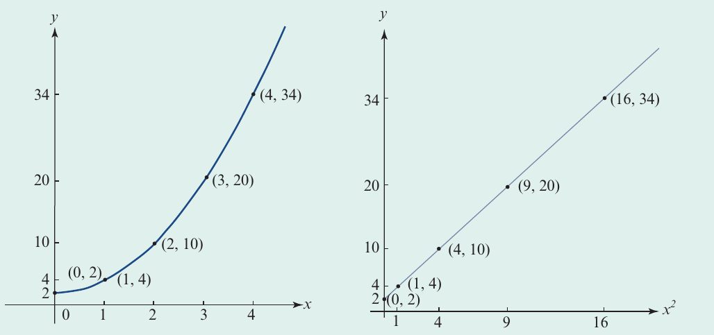
When data follows a quadratic pattern, squaring the $x$ -values before plotting can reveal a linear relationship. This means we transform our original $x$ -values into $x^2$ values and then plot $y$ against these new values.

What to do:

Calculate $x^2$ for each $x$ -value
Plot $y$ against $x^2$ (not against $x$ )
If the points form a straight line, the relationship follows the model $y = kx^2 + c$

Finding the equation

Once we've confirmed the transformed data is linear, we need to find two values:

k (the slope): Calculate using $\text{slope} = \frac{\text{rise}}{\text{run}}$
c (the y-intercept): Either read directly from the graph where $x^2 = 0$ , or substitute known values into the equation and solve

lightbulbExample

Worked Example: Modelling with $y = kx^2 + c$

Here's a dataset that has undergone an $x^2$ transformation:

$x$	0	1	2	3	4
$x^2$	0	1	4	9	16
$y$	2	4	10	20	34

Step 1: Find k by calculating the slope

Select any two points from the linearised graph (the right-hand graph where $y$ is plotted against $x^2$ ).

Let's use the points $(4, 10)$ and $(9, 20)$ :

$k = \text{slope} = \frac{\text{rise}}{\text{run}}$

$k = \frac{20 - 10}{9 - 4} = \frac{10}{5} = 2$

Step 2: Find c (the y-intercept)

Looking at the linearised graph, the line crosses the y-axis at $2$ , so c = 2.

Alternatively, we can substitute our known values into the equation:

$y = kx^2 + c$

Using the point where $x = 2$ and $y = 10$ :

$10 = 2(2^2) + c$

$10 = 8 + c$

$c = 2$

Step 3: Write the final equation

Substituting $k = 2$ and $c = 2$ :

$y = 2x^2 + 2$

Using the model $y = \frac{k}{x} + c$

Understanding the reciprocal transformation

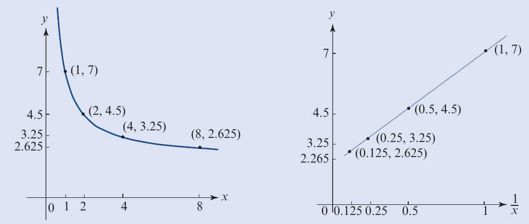
Some relationships show an inverse pattern where $y$ decreases as $x$ increases. For these, transforming $x$ -values to their reciprocals ( $\frac{1}{x}$ ) can reveal a linear relationship.

infoNote

What to do:

Calculate $\frac{1}{x}$ for each $x$ -value
Plot $y$ against $\frac{1}{x}$ (not against $x$ )
If the points form a straight line, the relationship follows the model $y = \frac{k}{x} + c$

Finding the equation

The process is similar to the previous model:

k (the slope): Calculate using $\text{slope} = \frac{\text{rise}}{\text{run}}$
c (the y-intercept): Substitute known values into $y = \frac{k}{x} + c$ and solve

lightbulbExample

Worked Example: Modelling with $y = \frac{k}{x} + c$

Here's a dataset that has undergone a $\frac{1}{x}$ transformation:

$x$	1	2	4	8
$\frac{1}{x}$	1	0.5	0.25	0.125
$y$	5	3	2	1.5

Step 1: Find k by calculating the slope

Select two points from the linearised graph. Let's use $(0.5, 3)$ and $(1, 5)$ :

$k = \text{slope} = \frac{\text{rise}}{\text{run}}$

$k = \frac{5 - 3}{1 - 0.5} = \frac{2}{0.5} = 4$

Step 2: Find c by substitution

Using the equation $y = \frac{k}{x} + c$ and the point where $x = 2$ and $y = 3$ :

$y = \frac{k}{x} + c$

$3 = \frac{4}{2} + c$

$3 = 2 + c$

$c = 1$

Step 3: Write the final equation

Substituting $k = 4$ and $c = 1$ :

$y = \frac{4}{x} + 1$

Using the model $y = k\log_{10}(x) + c$

Understanding the logarithmic transformation

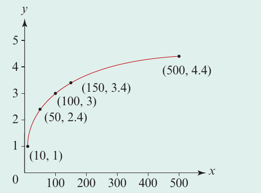
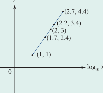
When data shows logarithmic growth (rapid increase initially, then slowing down), transforming $x$ -values using logarithms can reveal a linear relationship.

infoNote

What to do:

Calculate $\log_{10}(x)$ for each $x$ -value
Plot $y$ against $\log_{10}(x)$ (not against $x$ )
If the points form a straight line, the relationship follows the model $y = k\log_{10}(x) + c$

Finding the equation

Same approach as before:

k (the slope): Calculate using $\text{slope} = \frac{\text{rise}}{\text{run}}$
c (the y-intercept): Substitute known values into $y = k\log_{10}(x) + c$ and solve

lightbulbExample

Worked Example: Modelling with $y = k\log_{10}(x) + c$

Here's a dataset that has undergone a $\log_{10}(x)$ transformation:

$x$	10	50	100	150	500
$\log_{10}(x)$	1	1.7	2	2.2	2.7
$y$	1	2.4	3	3.4	4.4

Step 1: Find k by calculating the slope

Select two points from the linearised graph. Let's use $(1.7, 2.4)$ and $(2, 3)$ :

$k = \text{slope} = \frac{\text{rise}}{\text{run}}$

$k = \frac{3 - 2.4}{2 - 1.7} = \frac{0.6}{0.3} = 2$

Step 2: Find c by substitution

Using the equation $y = k\log_{10}(x) + c$ and the point where $x = 10$ and $y = 1$ :

$y = k\log_{10}(x) + c$

$1 = 2\log_{10}(10) + c$

Remember that $\log_{10}(10) = 1$ :

$1 = 2(1) + c$

$c = -1$

Step 3: Write the final equation

Substituting $k = 2$ and $c = -1$ :

$y = 2\log_{10}(x) - 1$

Exam tips

chatImportant

Critical Exam Strategies

Always transform first: Don't try to find the equation using the original $x$ -values. Always work with the transformed values ( $x^2$ , $\frac{1}{x}$ , or $\log_{10}(x)$ ).
Choose clear points: When calculating slope, select points with coordinates that are easy to read and calculate with.
Check your y-intercept: The y-intercept occurs where the horizontal axis equals zero. For $x^2$ transformations, this is straightforward. For $\frac{1}{x}$ and $\log_{10}(x)$ transformations, you may need to use substitution.
Use your calculator wisely: For logarithmic transformations, use your calculator's log function. Make sure you're using $\log_{10}$ (common logarithm), not natural logarithm.
Verify your answer: Substitute one of the original data points into your final equation to check it works.

Remember!

bookmarkSummary

Key Points to Remember:

Non-linear data can be modelled using three main transformations: $kx^2 + c$ , $\frac{k}{x} + c$ , and $k\log_{10}(x) + c$
The transformation determines what you plot on the horizontal axis: Plot $y$ against $x^2$ , $\frac{1}{x}$ , or $\log_{10}(x)$ respectively
In all three models, k is the slope and c is the y-intercept of the transformed (linear) graph
To find k: Calculate the slope of the straight-line graph using $\frac{\text{rise}}{\text{run}}$ with any two points on the line
To find c: Either read the y-intercept from the graph (where the transformed x-value equals zero) or substitute known values into the equation and solve

Further Modelling of Non-Linear Data (VCE SSCE General Mathematics): Revision Notes

Further Modelling of Non-Linear Data