Continuous Random Variables Revision Notes for VCE SSCE Mathematical Methods

Continuous Random Variables

Introduction to continuous random variables

A continuous random variable can assume any value within a specific interval on the real number line. Unlike discrete random variables that take distinct, separated values, continuous random variables have no gaps between possible values.

infoNote

The key difference between continuous and discrete random variables is that continuous variables can take any value within a range, while discrete variables take only specific, separated values.

For example, if $X$ represents the distance in metres that a parachutist lands from a marker, then $X$ is a continuous random variable. The values that $X$ can take are all non-negative real numbers.

An example of a continuous random variable

Continuous random variables have an important characteristic: they can be measured with unlimited precision, at least theoretically.

Consider a person's weight in kilograms. Let $W$ be the actual weight and $W_i$ be the weight measured to the $i$ th decimal place.

The table shows that:

$W_0 = 83$ implies $82.5 \leq W < 83.5$
$W_1 = 83.3$ implies $83.25 \leq W < 83.35$
$W_2 = 83.28$ implies $83.275 \leq W < 83.285$
$W_3 = 83.281$ implies $83.2805 \leq W < 83.2815$

This pattern continues indefinitely. Each measured value actually represents a range or interval.

Why point probabilities are zero

Because continuous random variables cannot take exact values (they are always rounded based on measurement precision), the probability of the variable equalling any specific value is zero.

chatImportant

For all continuous random variables:

\Pr(W = w) = 0 \text{ for all } w

This is a fundamental property that distinguishes continuous from discrete random variables. In practice, we work with probabilities over intervals instead of specific points.

For example:

\Pr(W_0 = 83) = \Pr(82.5 \leq W < 83.5)

To find this probability, we could measure the weights of many randomly chosen people and determine what proportion have weights in this interval.

From histograms to probability density functions

If we create a histogram of weights from a large sample, we might obtain something like this:

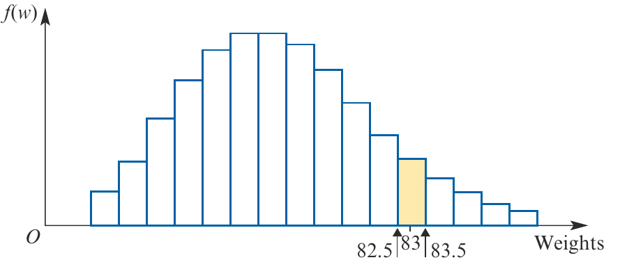
From this histogram:

\Pr(W_0 = 83) = \Pr(82.5 \leq W < 83.5) = \frac{\text{shaded area from 82.5 to 83.5}}{\text{total area}}

If we scale the histogram so that the total area under all blocks equals 1, then:

\Pr(W_0 = 83) = \text{area under block from 82.5 to 83.5}

infoNote

As we collect more data and use smaller class intervals, something remarkable happens: the histogram begins to transform into a smooth curve. This transition is fundamental to understanding continuous random variables.

Now imagine collecting more data and using smaller class intervals. As the sample size increases and the intervals become arbitrarily small, the histogram can be represented by a smooth curve:

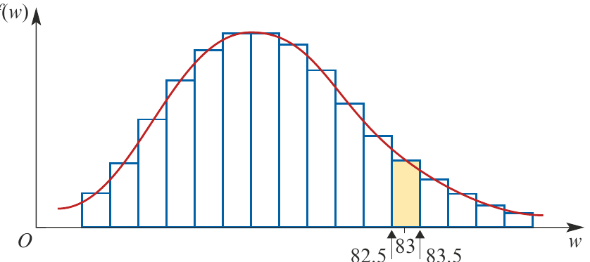
This smooth curve is fundamental to understanding continuous random variables.

Probability density functions

The function $f$ that represents the histogram as the number of intervals increases is called the probability density function (PDF). The probability density function describes the probability distribution of a continuous random variable $X$ .

With the smooth curve, probabilities are represented by areas under the curve rather than areas of histogram bars:

\Pr(W_0 = 83) = \Pr(82.5 \leq W < 83.5) = \int_{82.5}^{83.5} f(w) \, dw

Properties of probability density functions

chatImportant

Two Essential Properties of a Probability Density Function

A probability density function $f$ is a function with domain on some interval (such as $[c, d]$ or $\mathbb{R}$ ) that satisfies two conditions:

1. $f(x) \geq 0$ for all $x$ in the interval (the function is always non-negative)

2. The area under the graph of the function equals 1

If the domain of $f$ is $[c, d]$ , the second condition means:

\int_c^d f(x) \, dx = 1

For unbounded intervals, we use limits:

If the domain is $(1, \infty)$ : $\int_1^{\infty} f(x) \, dx = 1$ , computed as $\lim_{k \to \infty} \int_1^k f(x) \, dx$
If the domain is $\mathbb{R}$ : $\int_{-\infty}^{\infty} f(x) \, dx = 1$ , computed as $\lim_{k \to \infty} \int_{-k}^k f(x) \, dx$

infoNote

Definite integrals with one or both limits infinite are called improper integrals.

The probability density function of a random variable

Consider a continuous random variable $X$ with range $[c, d]$ (or an unbounded interval). Let $f$ be a probability density function with domain $[c, d]$ .

We say that $f$ is the probability density function of $X$ if:

\Pr(a < X < b) = \int_a^b f(x) \, dx

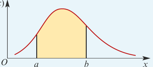
for all $a < b$ in the range of $X$ .

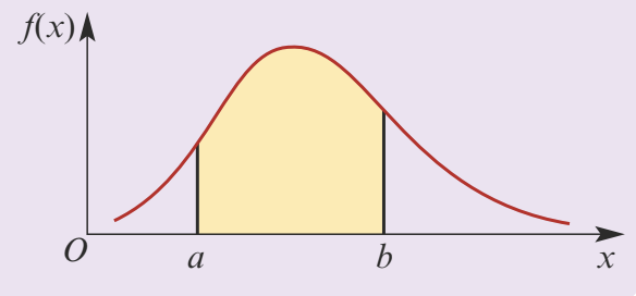
The shaded area represents the probability that $X$ falls between $a$ and $b$ .

Important notes

chatImportant

Critical Concepts About Probability Density Functions

The values of a probability density function are not probabilities themselves. The function $f(x)$ may take values greater than 1.
For continuous random variables, the probability of any specific value is 0: $\Pr(X = a) = 0$ .
Because point probabilities are zero, all of the following expressions have the same value:
- $\Pr(a < X < b)$
- $\Pr(a \leq X < b)$
- $\Pr(a < X \leq b)$
- $\Pr(a \leq X \leq b)$
If $f$ has domain $[c, d]$ and $a \in [c, d]$ , then $\Pr(X < a) = \Pr(X \leq a) = \int_c^a f(x) \, dx$

The natural extension of a probability density function

Any probability density function $f$ with domain $[c, d]$ can be extended to a function $f^*$ with domain $\mathbb{R}$ by defining:

f^*(x) = \begin{cases} f(x) & \text{if } x \in [c, d] \\ 0 & \text{if } x \notin [c, d] \end{cases}

This natural extension leads to a general form for the two properties:

1. $f(x) \geq 0$ for all $x$

2. $\int_{-\infty}^{\infty} f(x) \, dx = 1$

Probability density functions with unbounded domains

When working with unbounded intervals, we evaluate definite integrals using limits:

infoNote

Evaluating Improper Integrals

To integrate over $(-\infty, a)$ : find $\lim_{k \to -\infty} \int_k^a f(x) \, dx$
To integrate over $(a, \infty)$ : find $\lim_{k \to \infty} \int_a^k f(x) \, dx$
To integrate over $(-\infty, \infty)$ : find $\lim_{k \to \infty} \int_{-k}^k f(x) \, dx$

Worked examples

lightbulbExample

Worked Example: Finding the Constant in a PDF

Suppose the random variable $X$ has the probability density function:

f(x) = \begin{cases} cx & \text{if } 0 \leq x \leq 2 \\ 0 & \text{otherwise} \end{cases}

a Find the value of $c$ that makes $f$ a probability density function.

b Find $\Pr(X > 1.5)$ .

Solution

a Since $f$ is a probability density function, we know that $\int_{-\infty}^{\infty} f(x) \, dx = 1$ .

\int_{-\infty}^{\infty} f(x) \, dx = \int_0^2 cx \, dx \quad \text{since } f(x) = 0 \text{ elsewhere}

Therefore $2c = 1$ and so c = 0.5.

b $\Pr(X > 1.5) = \int_{1.5}^2 0.5x \, dx$

lightbulbExample

Worked Example: Verifying a PDF and Calculating Probabilities

Consider the function $f$ with the rule:

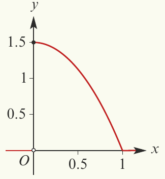
f(x) = \begin{cases} 1.5(1 - x^2) & \text{if } 0 \leq x \leq 1 \\ 0 & \text{otherwise} \end{cases}

a Sketch the graph of $f$ .

b Show that $f$ is a probability density function.

c Find $\Pr(X > 0.5)$ , where the random variable $X$ has probability density function $f$ .

Solution

a For $0 \leq x \leq 1$ , the graph of $y = f(x)$ is part of a parabola with intercepts at $(0, 1.5)$ and $(1, 0)$ .

b From the graph, we can see that f(x) ≥ 0 for all x, so the first condition holds.

The second condition to check is that $\int_{-\infty}^{\infty} f(x) \, dx = 1$ .

\int_{-\infty}^{\infty} f(x) \, dx = \int_0^1 1.5(1 - x^2) \, dx \quad \text{since } f(x) = 0 \text{ elsewhere}

Thus the second condition holds, and hence f is a probability density function.

c $\Pr(X > 0.5) = \int_{0.5}^1 1.5(1 - x^2) \, dx$

lightbulbExample

Worked Example: Exponential Probability Density Function

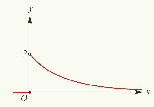
Consider the exponential probability density function $f$ with the rule:

f(x) = \begin{cases} 2e^{-2x} & x > 0 \\ 0 & x \leq 0 \end{cases}

a Sketch the graph of $f$ .

b Show that $f$ is a probability density function.

c Find $\Pr(X > 1)$ , where the random variable $X$ has probability density function $f$ .

Solution

a For $x > 0$ , the graph of $y = f(x)$ is part of an exponential function with $y$ -axis intercept 2. As $x \to \infty$ , $y \to 0$ .

b Since f(x) ≥ 0 for all x, the first condition holds.

The second condition to check is that $\int_{-\infty}^{\infty} f(x) \, dx = 1$ .

\int_{-\infty}^{\infty} f(x) \, dx = \int_0^{\infty} 2e^{-2x} \, dx \quad \text{since } f(x) = 0 \text{ elsewhere}

Thus $f$ satisfies the two conditions for a probability density function.

c $\Pr(X > 1) = \lim_{k \to \infty} \int_1^k 2e^{-2x} \, dx$

(correct to four decimal places)

lightbulbExample

Worked Example: Conditional Probability

The time (in seconds) that it takes a student to complete a puzzle is a random variable $X$ with a density function given by:

f(x) = \begin{cases} \frac{5}{x^2} & x \geq 5 \\ 0 & x < 5 \end{cases}

a Find the probability that a student takes less than 12 seconds to complete the puzzle.

b Find the probability that a student takes between 8 and 10 seconds to complete the puzzle, given that they take less than 12 seconds.

Solution

a $\Pr(X < 12) = \int_5^{12} f(x) \, dx$

b $\Pr(8 < X < 10 \mid X < 12) = \frac{\Pr(8 < X < 10 \cap X < 12)}{\Pr(X < 12)}$

bookmarkSummary

Key Points to Remember

A continuous random variable can take any value within an interval of real numbers.
For continuous random variables, $\Pr(X = a) = 0$ for any specific value $a$ . We work with probabilities over intervals instead.
A probability density function must satisfy two properties:
1. $f(x) \geq 0$ for all $x$ (always non-negative)
2. $\int_{-\infty}^{\infty} f(x) \, dx = 1$ (total area equals 1)
Probabilities are calculated as areas under the PDF curve: $\Pr(a < X < b) = \int_a^b f(x) \, dx$
For unbounded domains, we use improper integrals evaluated as limits.

Continuous Random Variables (VCE SSCE Mathematical Methods): Revision Notes