Cumulative Distribution Functions (VCE SSCE Mathematical Methods): Revision Notes

Cumulative Distribution Functions

What is a cumulative distribution function?

The cumulative distribution function (often abbreviated as CDF) is another important way to describe a continuous random variable. While the probability density function (PDF) tells us about the distribution of probabilities, the CDF tells us about accumulated probabilities up to a certain point.

For a continuous random variable $X$ with probability density function $f$ defined on the interval $[c, d]$, the cumulative distribution function $F$ is defined as:

$$F(x) = \text{Pr}(X \leq x)$$ $$= \int_c^x f(t) \, dt$$

where $t$ is the variable of integration.

Understanding the formula

Let's break down what this formula means:

• $F(x)$ represents the cumulative distribution function evaluated at $x$
• $\text{Pr}(X \leq x)$ is the probability that our random variable is at most $x$
• The integral $\int_c^x f(t) \, dt$ calculates the area under the probability density function from the lower bound $c$ up to the value $x$
• We use $t$ as the variable of integration (rather than $x$) because $x$ appears as the upper limit of the integral

Visualizing the relationship between PDF and CDF

The diagram below illustrates the connection between the probability density function and the cumulative distribution function:

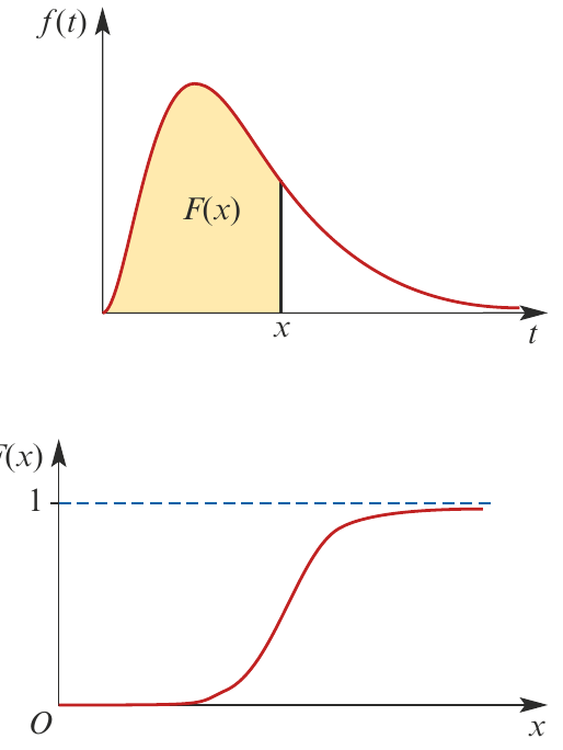
The top panel shows the probability density function $f(t)$. The shaded yellow area under the curve from the lower bound (in this case, 0) up to the value $x$ represents $F(x)$.

The bottom panel shows the corresponding cumulative distribution function $F(x)$. Notice how it:

• Starts near 0 at the origin
• Increases in an S-shaped curve
• Approaches 1 asymptotically (shown by the horizontal dashed line)

Properties of cumulative distribution functions

There are three fundamental properties that every cumulative distribution function must satisfy. For a continuous random variable $X$ with domain $[c, d]$:

Property 1: The CDF starts at zero

$$F(c) = 0$$

At the lower bound of the domain, the probability that $X$ takes a value less than or equal to $c$ is 0. This makes sense because $c$ is the smallest possible value.

Property 2: The CDF ends at one

$$F(d) = 1$$

At the upper bound of the domain, the probability that $X$ takes a value less than or equal to $d$ is 1. This is certain because $d$ is the largest possible value.

Property 3: The CDF never decreases

If $x_1 \leq x_2$, then $\text{Pr}(X \leq x_1) \leq \text{Pr}(X \leq x_2)$

In other words: $x_1 \leq x_2$ implies $F(x_1) \leq F(x_2)$

This means $F$ is a non-decreasing function. As $x$ increases, the cumulative probability either stays the same or increases, but it never decreases. This is logical because we're accumulating more probability as we move to larger values of $x$.

Connection to the probability density function

There's an important mathematical relationship between the CDF and the PDF:

The cumulative distribution function is always continuous for any continuous random variable $X$.

Using the fundamental theorem of calculus, we can show that the derivative of the cumulative distribution function equals the probability density function:

$$F'(x) = f(x)$$

This holds for each value of $x$ where $f$ is continuous. This relationship tells us that:

• Integrating the PDF gives us the CDF
• Differentiating the CDF gives us the PDF

CDFs for probability density functions defined on all real numbers

When the probability density function is defined on all real numbers (denoted by $\mathbb{R}$), the cumulative distribution function is given by:

$$F(x) = \text{Pr}(X \leq x)$$ $$= \int_{-\infty}^x f(t) \, dt$$

In this case, the integral extends from negative infinity up to $x$. The properties are slightly modified:

• $F(x) \to 0$ as $x \to -\infty$
• $F(x) \to 1$ as $x \to \infty$

Worked example

Remember!