Linear Models (VCE SSCE Mathematical Methods): Revision Notes
Linear Models
Introduction to linear models
Linear models help us represent real-world situations where one quantity changes at a constant rate relative to another quantity. These models appear frequently in everyday scenarios such as calculating costs, measuring distances over time, or tracking growth patterns.
A linear model takes the form of a straight-line equation, typically written as:
where:
- represents the gradient (rate of change)
- represents the y-intercept (starting value)
The equation is the foundation of all linear models. Understanding each component helps you interpret real-world situations: the gradient tells you how quickly things change, while the y-intercept tells you the starting value.
Cost functions
A cost function is a type of linear model that describes how total costs depend on the quantity of items or services. Cost functions typically combine two components:
Fixed costs: A constant amount that doesn't change regardless of quantity (represented by the y-intercept)
Variable costs: An amount that increases with each additional unit (represented by the gradient multiplied by the quantity)
The general form of a cost function is:
Worked Example: Historical Site Entrance Fees
A historical site charges a tour company for priority entrance. The charge consists of a monthly fee of $200 plus $3.50 for each tourist brought to the site. We need to construct a cost function and sketch the graph.
Setting up the function:
Let = monthly charge in dollars
Let = number of tourists
The cost function is:
In this function:
- The fixed monthly fee is $200 (the y-intercept)
- Each tourist adds $3.50 to the cost (the gradient)
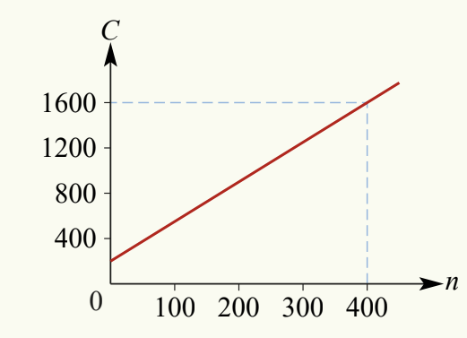
Since the number of tourists must be a whole number (you can't have 2.5 tourists!), the graph should technically consist of separate points rather than a continuous line. However, at this scale, it's more practical to show it as a continuous line for clarity.
Distance-time relationships
Another important application of linear models involves the relationship between distance travelled and time when an object moves at constant speed.
Constant speed creates linear relationships
When an object travels at a constant speed, the distance it covers increases steadily with time. This creates a linear relationship.
For example, if a car travels at 40 km/h, the relationship between distance travelled ( kilometres) and time taken ( hours) is:
The graph of against is a straight line through the origin. The gradient of this line is 40, which represents the speed in kilometres per hour.
Worked Example: Car Travelling on Highway
A car starts from point A on a highway, located 10 kilometres past the Wangaratta post office. The car travels at a constant speed of 90 km/h towards picnic stop B, which is 120 kilometres further along from A. Let hours be the time after the car leaves point A.
Part a: Distance from the post office
At time , the car has travelled kilometres from point A. Since point A is already 10 kilometres past the post office, the distance from the post office is:
Part b: Distance from point B
Point B is 120 kilometres from A. As the car travels towards B, it gets closer, so the remaining distance decreases. At time , the car has covered kilometres towards B, leaving:
Part c: Graphs and gradients
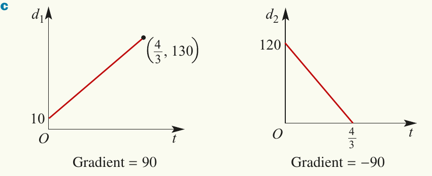
The left graph shows versus . It has a gradient of 90, which is positive because the car is moving away from the post office.
The right graph shows versus . It has a gradient of -90, which is negative because the car is moving towards point B (the distance is decreasing).
In distance-time graphs, the sign of the gradient tells you the direction of movement:
- Positive gradient: Moving away from the reference point
- Negative gradient: Moving towards the reference point
- Magnitude of gradient: The speed (always positive)
Interpreting gradients in linear models
The gradient of a linear model tells us the rate of change. Its interpretation depends on the context:
In cost functions: The gradient represents the cost per additional unit. A positive gradient means costs increase as quantity increases.
In distance-time relationships: The gradient represents speed.
- A positive gradient means the object is moving away from the reference point (distance increasing)
- A negative gradient means the object is moving towards the reference point (distance decreasing)
- The magnitude (size) of the gradient tells us how fast the object is moving
In general:
- Positive gradient = increasing relationship
- Negative gradient = decreasing relationship
- Larger magnitude of gradient = steeper change
Common Mistake to Avoid:
Students often confuse a negative gradient with negative speed. Remember: speed is always positive! A negative gradient in a distance-time graph simply means the distance is decreasing (moving towards a reference point), but the speed itself is the magnitude of the gradient.
Key Points to Remember:
- Linear models represent situations where one quantity changes at a constant rate with respect to another
- Cost functions combine fixed costs (y-intercept) and variable costs (gradient × quantity)
- In distance-time graphs with constant speed, the gradient equals the speed
- Positive gradients indicate movement away from a reference point or increasing values
- Negative gradients indicate movement towards a reference point or decreasing values
- The magnitude of the gradient tells you the rate of change (e.g., speed in km/h, cost per unit)