Analysing Motion Through Graphs Revision Notes for VCE SSCE Physics

Analysing Motion Through Graphs

Introduction to motion graphs

Motion graphs are powerful tools for analysing and understanding how objects move. This topic focuses on three main types of graphs used in physics to represent motion:

Displacement-time graphs
Velocity-time graphs
Acceleration-time graphs

Each type of graph provides different information about an object's motion. Understanding how to read, interpret, and extract information from these graphs is essential for analysing both uniform and non-uniform motion in a straight line.

infoNote

Motion graphs provide a visual representation of an object's movement over time. By analysing the shape, gradient, and area of these graphs, we can determine key information such as velocity, acceleration, and displacement without complex calculations.

Vector quantities of motion

Distance versus displacement

Distance is a scalar quantity that measures the total path length travelled by an object. It only requires a magnitude (how much ground was covered).

Displacement is a vector quantity that measures the straight-line distance from the starting position (origin) to the final position. It requires both magnitude and direction.

lightbulbExample

Example: Hiker's Journey

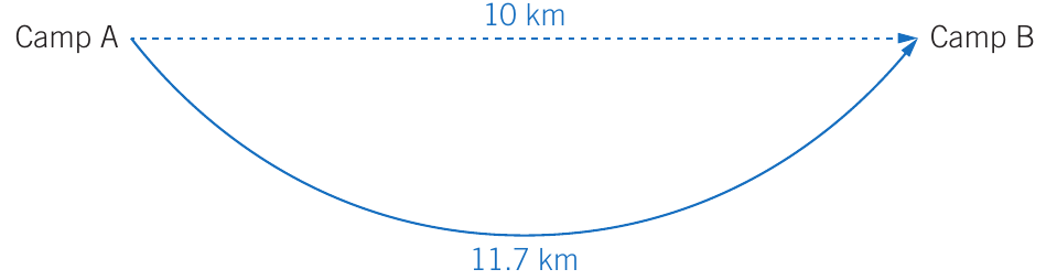
A hiker walks from Camp A to Camp B. The camps are separated by a straight-line distance of 10 km when travelling directly east. However, a mountain blocks the direct path, so the hiker must walk 11.7 km around the mountain.

Displacement: 10 km east (straight-line distance)
Distance: 11.7 km (actual path travelled)

chatImportant

Key point: When an object returns to its starting position, its displacement is zero, even though it has travelled a non-zero distance. This is because displacement only measures the net change in position from start to finish.

lightbulbExample

Worked Example: Track Runner

A track runner completes exactly four laps of a 500 m circular track, finishing where they started.

Distance travelled: $500 \times 4 = 2000$ m

Displacement: 0 m (the runner finishes at the origin, so there is no net change in position)

Speed versus velocity

Speed is the rate of change of distance. It is a scalar quantity requiring only a magnitude. The formula for average speed is:

$\text{average speed} = \frac{\Delta d}{\Delta t}$

Where:

$\Delta d$ = change in distance (m)
$\Delta t$ = change in time (s)

Velocity is the rate of change of displacement. It is a vector quantity requiring both magnitude and direction. The direction of velocity is the same as the direction of displacement change. The formula for average velocity is:

$v_{av} = \frac{\Delta s}{\Delta t}$

Where:

$v_{av}$ = average velocity (m s⁻¹)
$\Delta s$ = change in displacement (m)
$\Delta t$ = change in time (s)

chatImportant

Important distinction: Velocity can be positive or negative, depending on the direction of motion relative to the chosen coordinate system. A velocity of 10 m s⁻¹ north means the object is moving 10 m further north every second.

Converting between units

Speed and velocity are often given in kilometres per hour (km h⁻¹), but in physics calculations it's usually necessary to convert to metres per second (m s⁻¹).

chatImportant

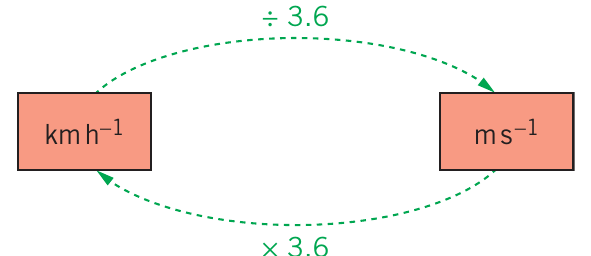
Conversion rules:

To convert from km h⁻¹ to m s⁻¹: divide by 3.6
To convert from m s⁻¹ to km h⁻¹: multiply by 3.6

lightbulbExample

Example: Converting Units

Convert 72 km h⁻¹ to m s⁻¹:

$72 \div 3.6 = 20 \text{ m s}^{-1}$

Acceleration

Acceleration is the rate of change of velocity. It is a vector quantity with the symbol $a$ . The SI unit for acceleration is metres per second per second (m s⁻²), which means "metres per second, per second".

$a = \frac{\Delta v}{\Delta t} = \frac{v - u}{t}$

Where:

$a$ = acceleration (m s⁻²)
$\Delta v$ = change in velocity (m s⁻¹)
$v$ = final velocity (m s⁻¹)
$u$ = initial velocity (m s⁻¹)
$t$ = time (s)

infoNote

Understanding acceleration: If a car starting from rest accelerates at 4 m s⁻² in a straight line:

After 1 second, the car's velocity is 4 m s⁻¹
After 2 seconds, the car's velocity is 8 m s⁻¹
After 3 seconds, the car's velocity is 12 m s⁻¹

The velocity increases by 4 m s⁻¹ every second.

Acceleration due to gravity: On Earth, objects in free fall (ignoring air resistance) accelerate downward at approximately 9.8 m s⁻². This is equivalent to the object's speed increasing by 35.3 km h⁻¹ every second.

infoNote

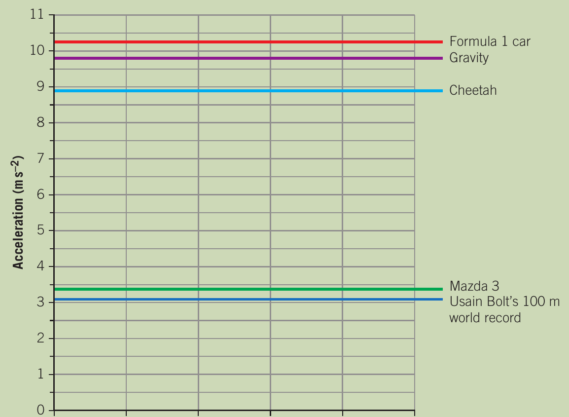
The graph shows that gravity produces an acceleration comparable to high-performance vehicles. A Formula 1 car can accelerate at about 10 m s⁻², only slightly more than gravitational acceleration.

Displacement-time graphs

Displacement-time graphs show how far an object is from its origin at any given point in time. The displacement is plotted on the y-axis and time on the x-axis.

This graph shows a jogger who:

Runs away from home for 20 seconds, covering 80 m
Stops and rests for 24 seconds
Runs back toward home for 12 seconds, covering the 80 m
Continues running in the opposite direction for another 20 seconds, covering 80 m

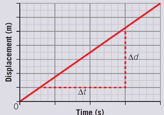
Gradient of displacement-time graphs

The gradient (or slope) of a line is calculated as:

$\text{gradient} = \frac{\text{rise}}{\text{run}}$

For a displacement-time graph:

$\text{gradient} = \frac{\Delta s}{\Delta t} = v$

chatImportant

Key principle: The gradient of a displacement-time graph gives the velocity of the object.

lightbulbExample

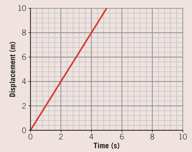
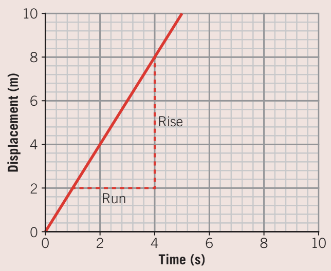
Worked Example: Finding Velocity from Gradient

A body moves from rest in a straight line. What is the gradient of the displacement-time graph shown?

Solution: Take two clear points from the line and calculate:

$\text{gradient} = \frac{\text{rise}}{\text{run}} = \frac{8 - 2}{4 - 1} = \frac{6}{3} = 2$

Since we're dividing displacement (m) by time (s), the unit is m s⁻¹.

Therefore: The gradient represents velocity, and the velocity is 2 m s⁻¹.

Interpreting different gradients

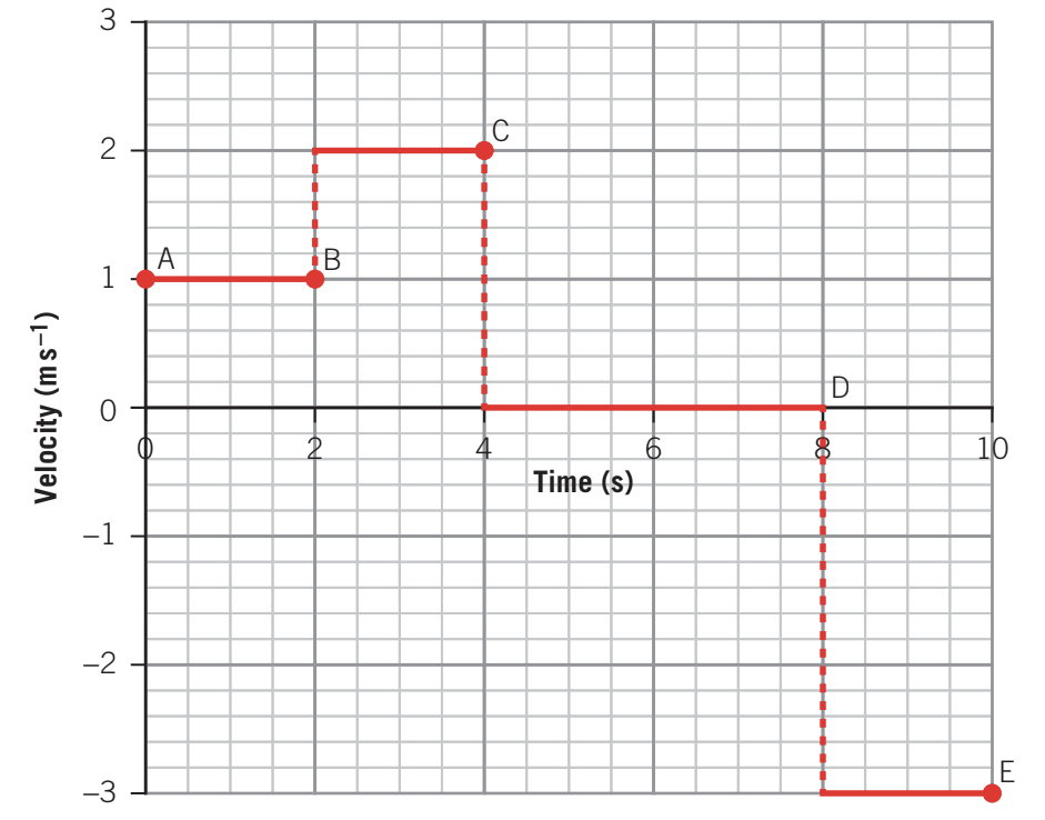
Consider the motion shown in this velocity-time graph with points A through E:

Positive gradient: Object moving away from origin (forward motion)
Zero gradient (horizontal line): Object is stationary (velocity = 0)
Negative gradient: Object moving toward origin (backward motion)
Steeper gradient: Faster velocity (greater rate of change of displacement)

Relationship between displacement-time and velocity-time graphs

The velocity-time graph can be derived from a displacement-time graph by plotting the gradient at each point in time.

lightbulbExample

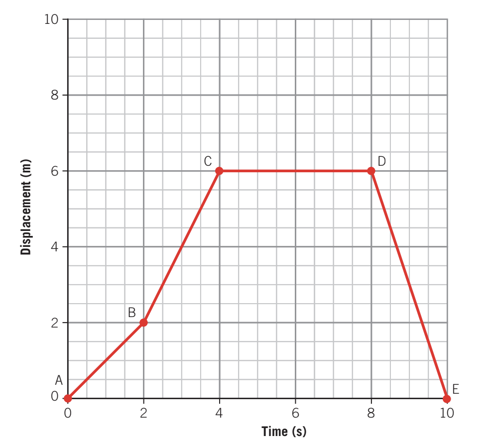
Example Interpretation:

From the displacement-time graph:

Section A to B: Constant positive gradient → constant positive velocity (1 m s⁻¹)
Section B to C: Steeper constant gradient → higher constant positive velocity (2 m s⁻¹)
Section C to D: Zero gradient (flat line) → zero velocity (stationary)
Section D to E: Negative constant gradient → constant negative velocity (-3 m s⁻¹)

The corresponding velocity-time graph shows these values as horizontal lines at different heights, with vertical jumps representing instantaneous velocity changes.

Velocity-time graphs

Velocity-time graphs display the velocity of an object at any given point in time. Velocity is plotted on the y-axis and time on the x-axis.

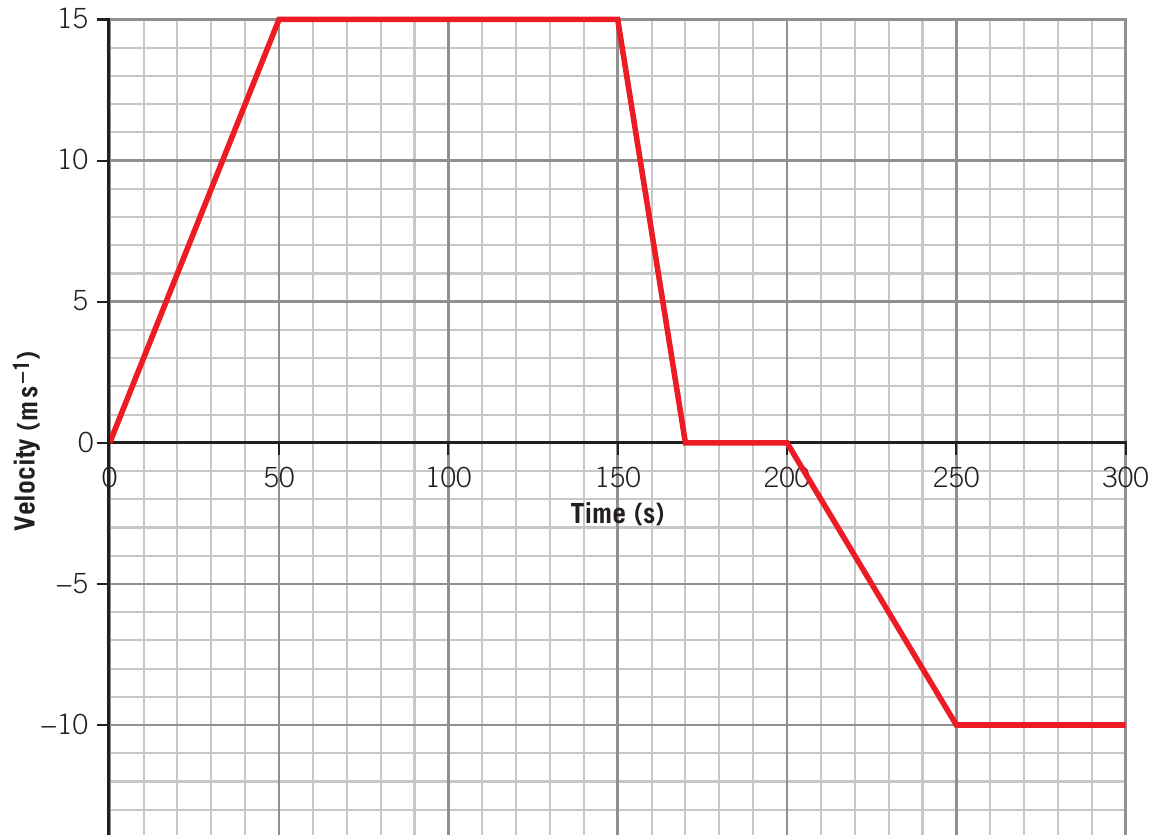
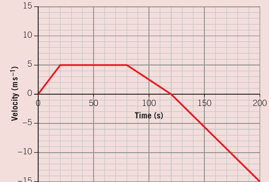
This graph shows a car's motion over 300 seconds, including:

Initial acceleration phase (velocity increasing)
Constant velocity phase (horizontal line at 15 m s⁻¹)
Deceleration phase (velocity decreasing to zero)
Constant velocity at zero (stationary)
Acceleration in the opposite direction (negative velocity increasing in magnitude)
Constant negative velocity (motion in reverse direction)

Gradient of velocity-time graphs

For a velocity-time graph:

$\text{gradient} = \frac{\text{rise}}{\text{run}} = \frac{\Delta v}{\Delta t} = a$

chatImportant

Key principle: The gradient of a velocity-time graph gives the acceleration of the object.

The unit is derived from dividing velocity (m s⁻¹) by time (s):

$\frac{\text{m s}^{-1}}{\text{s}} = \text{m s}^{-2}$

lightbulbExample

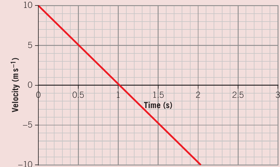
Worked Example: Ball Thrown Upward

A ball is thrown vertically upward with an initial velocity of 10 m s⁻¹. The velocity-time graph shows the ball's motion (ignoring air resistance).

Question a: When the velocity is zero (at $t = 1.02$ s), what is the significance?

Answer: The ball is at its maximum height. At this point, the ball has stopped moving upward and is about to begin falling downward.

Question b: Calculate the gradient and explain its significance.

Solution: $\text{gradient} = \frac{\text{rise}}{\text{run}} = \frac{0 - 10}{1.02 - 0} = -9.8 \text{ m s}^{-2}$

This gradient represents the acceleration due to gravity. The negative value indicates the acceleration is directed downward. This acceleration acts throughout the ball's flight, first slowing it down (when moving upward), then speeding it up (when moving downward).

Area under velocity-time graphs

chatImportant

Key principle: The area under a velocity-time graph represents the change in displacement.

For constant velocity over a time interval:

$\text{area} = \Delta s = v \times t$

lightbulbExample

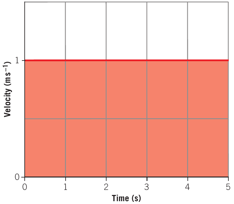
Simple Example: Constant Velocity

A hiker walks at a constant velocity of 1 m s⁻¹ for 5 seconds.

$\text{area} = \Delta s = 1 \times 5 = 5 \text{ m}$

The hiker's displacement is 5 m.

infoNote

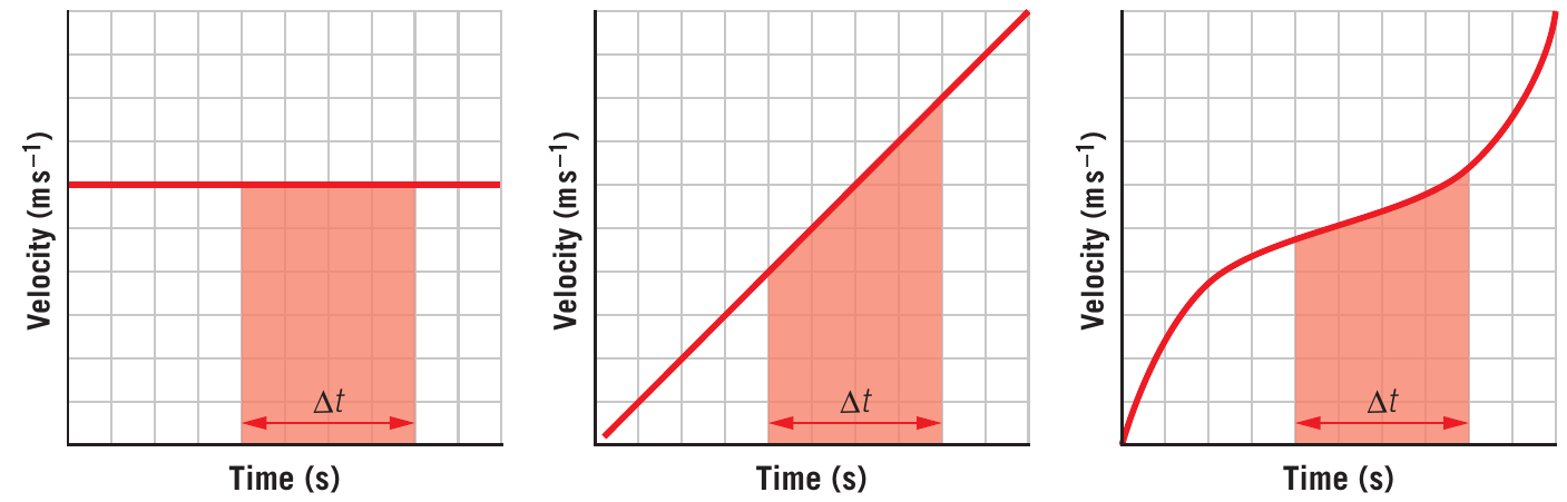
Important: This principle applies even when velocity is not constant. The area under the curve (whether it's a rectangle, triangle, trapezoid, or more complex shape) always gives the change in displacement.

Calculating areas for complex velocity-time graphs

When velocity changes, divide the graph into simple geometric shapes (rectangles and triangles), calculate the area of each, and add them together.

lightbulbExample

Worked Example: Cyclist Journey

A cyclist rides north, turns around, and returns to the starting point. Find:

a) Displacement after 120 s

Divide the graph into shapes and calculate areas:

$\text{Area} = \frac{1}{2}(20)(5) + (60)(5) + \frac{1}{2}(40)(5)$

$= 50 + 300 + 100 = 450 \text{ m}$

The displacement is 450 m north.

b) Displacement after 180 s

The graph now includes negative velocity (motion southward). Calculate the negative area:

$\text{Area (negative)} = \frac{1}{2}(60)(-15) = -450 \text{ m}$

The negative sign indicates southward displacement.

Total displacement: $450 + (-450) = 0$ m

The cyclist has returned to the starting position.

c) Total distance covered after 180 s

Distance is a scalar (no direction), so use the magnitude of all areas:

$\text{Distance} = 450 + 450 = 900 \text{ m}$

chatImportant

Key distinction: Displacement considers direction (vectors can cancel), while distance does not (always positive and cumulative).

Acceleration-time graphs

Acceleration-time graphs display the acceleration of an object at any given point in time. Acceleration is plotted on the y-axis and time on the x-axis.

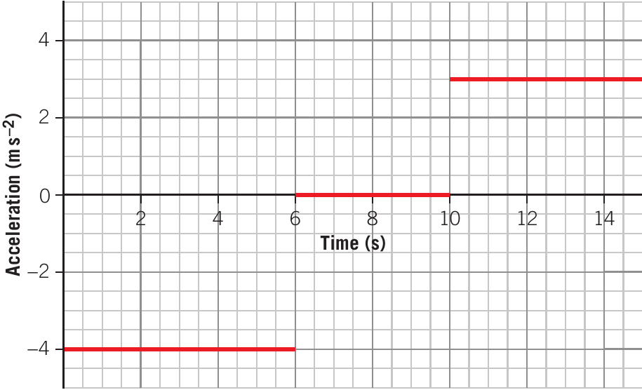
This graph shows a car braking:

From 0 to 6 s: constant negative acceleration of -4 m s⁻² (braking/decelerating)
From 6 to 10 s: zero acceleration (stationary or constant velocity)
From 10 to 15 s: constant positive acceleration of approximately +3 m s⁻² (accelerating forward)

infoNote

The negative acceleration doesn't necessarily mean the car is moving backward; it means the acceleration is in the opposite direction to the initial velocity (slowing down).

Area under acceleration-time graphs

chatImportant

Key principle: The area under an acceleration-time graph represents the change in velocity.

$\text{area} = \Delta v = a \times t$

The unit is derived from multiplying acceleration (m s⁻²) by time (s):

$\text{m s}^{-2} \times \text{s} = \text{m s}^{-1}$

lightbulbExample

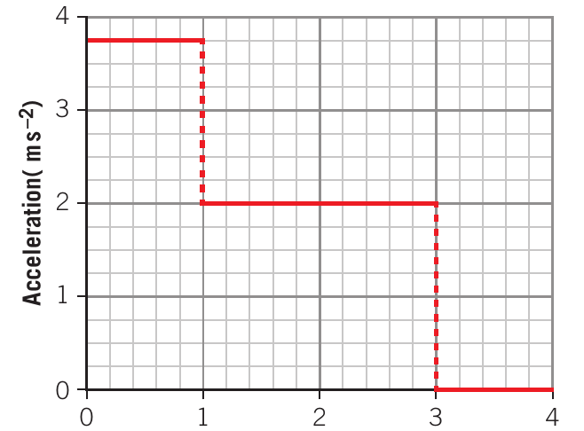
Worked Example: Car Approaching Roadworks

A car initially travelling at 72 km h⁻¹ approaches roadworks, slows down, passes through, and then accelerates again.

a) Calculate the speed through the roadworks (in km h⁻¹)

First, convert the initial velocity: $\text{Initial velocity} = \frac{72}{3.6} = 20 \text{ m s}^{-1}$

Calculate the change in velocity (area under graph from 0 to 8 s): $\Delta v = (-1)(8) = -8 \text{ m s}^{-1}$

Final velocity through roadworks: $v = 20 - 8 = 12 \text{ m s}^{-1}$

Convert to km h⁻¹: $12 \times 3.6 = 43.2 \text{ km h}^{-1}$

Answer: 43.2 km h⁻¹

b) Calculate the speed at the end of 50 s (in km h⁻¹)

From part (a), we know the velocity at 42 s is 12 m s⁻¹. Calculate the change from 42 s to 50 s:

$\Delta v = (2)(8) = 16 \text{ m s}^{-1}$

Final velocity: $v = 12 + 16 = 28 \text{ m s}^{-1}$

Convert to km h⁻¹: $28 \times 3.6 = 101 \text{ km h}^{-1}$

Answer: 101 km h⁻¹

Instantaneous versus average velocity

Average velocity

Average velocity is calculated over a time interval using:

$v_{av} = \frac{\Delta s}{\Delta t}$

This gives the overall rate of displacement change, but doesn't tell you the velocity at any specific moment.

lightbulbExample

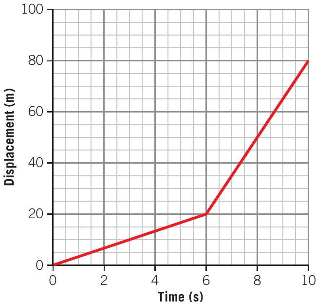
Example: Different Time Intervals

For a displacement-time graph showing curved motion (acceleration), different time intervals give different average velocities:

From 0 to 6 s: $v_{av} = \frac{20 - 0}{6 - 0} = 3.33$ m s⁻¹
From 6 to 10 s: $v_{av} = \frac{80 - 20}{10 - 6} = 15$ m s⁻¹
From 0 to 10 s: $v_{av} = \frac{80 - 0}{10 - 0} = 8$ m s⁻¹

Instantaneous velocity

Instantaneous velocity is the velocity at a specific point in time. On a displacement-time graph, it equals the gradient of the tangent line at that point.

chatImportant

Key difference:

Average velocity: Calculated over a time interval; gives the overall rate of change
Instantaneous velocity: Velocity at a specific moment; given by the gradient of the tangent

As the time interval becomes smaller and approaches zero, the average velocity approaches the instantaneous velocity.

infoNote

Practical note: Any real-world measurement of velocity is technically an average over some small time interval, because we must measure displacement over some finite time period. However, by making the time interval very small, we can get very close to the true instantaneous velocity.

Skills: Understanding and using gradients

What is a gradient?

The gradient measures the steepness of a graph. It's calculated as:

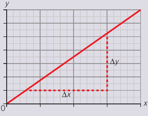
$\text{gradient} = \frac{\Delta y}{\Delta x} = \frac{\text{rise}}{\text{run}}$

chatImportant

The unit for the gradient is always the y-axis unit divided by the x-axis unit.

Gradient of displacement-time graphs

For a displacement-time graph:

$\text{gradient} = \frac{\Delta d}{\Delta t}$

Unit: $\frac{\text{m}}{\text{s}} = \text{m s}^{-1}$

Meaning: The gradient represents velocity.

Using gradients to determine relationships

lightbulbExample

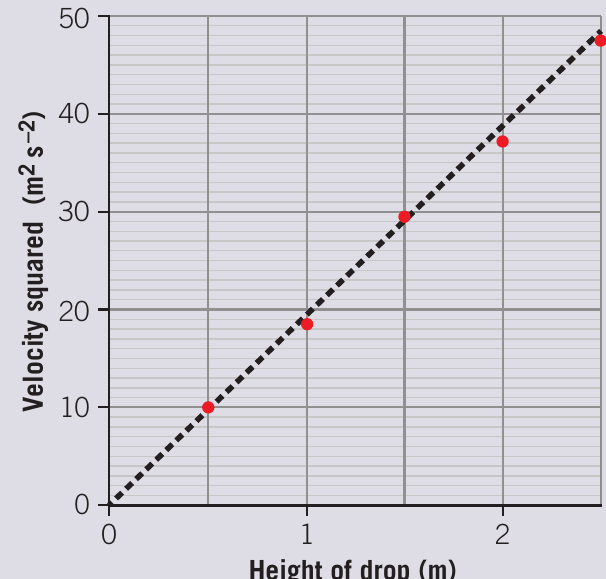
Worked Example: Experimental Determination of Gravitational Acceleration

Students drop a ball from different heights and measure its final velocity. They graph height of drop ( $s$ ) on the x-axis and velocity squared ( $v^2$ ) on the y-axis to test the equation:

$v^2 = u^2 + 2as$

Since initial velocity $u = 0$ :

$a = \frac{v^2}{2s}$

a) Determine the gradient (with unit)

Take two well-separated points:

$\text{gradient} = \frac{\text{rise}}{\text{run}} = \frac{48 - 0}{2.5 - 0} = 19.2$

Unit: $\frac{\text{m}^2 \text{s}^{-2}}{\text{m}} = \text{m s}^{-2}$

Gradient: 19.2 m s⁻²

b) Use the gradient to find acceleration due to gravity

Recognize that the gradient represents:

$\text{gradient} = \frac{v^2}{s}$

From the equation:

$a = \frac{v^2}{2s} = \frac{1}{2} \times \text{gradient}$

$a = \frac{1}{2} \times 19.2 = 9.6 \text{ m s}^{-2}$

The experimental value for gravitational acceleration is 9.6 m s⁻², which is close to the accepted value of 9.8 m s⁻². The small difference could be due to air resistance or measurement uncertainties.

Summary of graph interpretations

Graph Type	Gradient Represents	Area Under Graph Represents
Displacement-Time	Velocity	Not typically used
Velocity-Time	Acceleration	Change in displacement
Acceleration-Time	Rate of change of acceleration	Change in velocity

infoNote

Key tips for exam success:

Always identify what's on each axis before interpreting a graph
Check units carefully when calculating gradients or areas
Remember that negative values indicate direction, not "backwards" motion necessarily
For areas, divide complex shapes into rectangles and triangles
Pay attention to whether a question asks for distance (scalar) or displacement (vector)

bookmarkSummary

Key Points to Remember:

Displacement is a vector (requires direction); distance is a scalar (magnitude only)
Velocity is a vector (requires direction); speed is a scalar (magnitude only)
To convert km h⁻¹ to m s⁻¹, divide by 3.6; to convert m s⁻¹ to km h⁻¹, multiply by 3.6
The gradient of a displacement-time graph gives velocity
The gradient of a velocity-time graph gives acceleration
The area under a velocity-time graph gives change in displacement
The area under an acceleration-time graph gives change in velocity
When calculating areas with negative velocities, keep the negative sign for displacement but use magnitude for distance

Analysing Motion Through Graphs (VCE SSCE Physics): Revision Notes