Continuous Distributions 1 Revision Notes for AQA A-Level Further Maths

Continuous Distributions 1

Introduction to probability density functions

When working with discrete random variables, you can list all possible values and their associated probabilities in a probability distribution function. However, this approach does not work for continuous random variables because there are infinitely many possible values within any interval. Just as histograms replace bar charts for continuous data, probability density functions replace probability distribution functions for continuous variables.

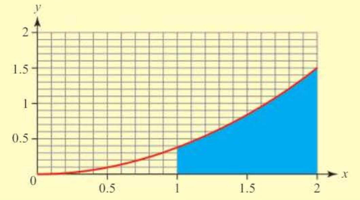
A probability density function (pdf) is a mathematical function that describes the likelihood of a continuous random variable taking values within a specific range. Instead of calculating probabilities for exact values, you find the probability that the variable falls between two values by calculating the area under the pdf curve between those points. This area is found using integration.

chatImportant

Definition: If $X$ is a random variable with probability density function $f(x)$ , then the probability that $X$ lies between values $a$ and $b$ is given by:

$P\{a < X < b\} = \int_{a}^{b} f(x)\,dx$

The area under the curve represents probability, which is similar to how area represents frequency in histograms. For continuous distributions, the probability of $X$ taking any single exact value is zero, so $P\{X = x\} = 0$ .

infoNote

This is a fundamental difference from discrete distributions: in continuous distributions, we cannot find the probability of an exact value, only the probability of falling within a range of values.

Properties of probability density functions

For a function to be a valid probability density function, it must satisfy two essential conditions. These properties ensure that the function represents a valid probability model.

chatImportant

Key properties:

Non-negativity: The function must be non-negative for all values in its domain: $f(x) \geq 0$

This means all probabilities are greater than or equal to zero.
Total probability equals one: The total area under the pdf curve must equal 1:

$\int_{-\infty}^{+\infty} f(x)\,dx = 1$

This represents the fact that the total probability of all possible outcomes is 1.

Worked example 1: verifying a valid pdf

lightbulbExample

Worked Example: Verifying a Valid PDF

A random variable $X$ has probability density function:

$f(x) = \begin{cases} \frac{3}{8}x^2 & \text{for } 0 < x < 2 \\ 0 & \text{otherwise} \end{cases}$

Part a: Sketch the curve $y = f(x)$ and verify that $f(x)$ is a valid pdf. Shade the area representing $P\{X > 1\}$ .

Part b: Find the value of $P\{X > 1\}$ .

Solution:

First, check the non-negativity condition. Since $f(x) = \frac{3}{8}x^2$ for $0 < x < 2$ , and this is always positive in the given range, the first property is satisfied.

Next, verify the total probability condition:

$\int_{0}^{2} \frac{3}{8}x^2\,dx = \left[\frac{x^3}{8}\right]_0^2 = \frac{8}{8} - 0 = 1$

Since both properties are satisfied, $f(x)$ is a valid pdf.

For part b:

$P\{X > 1\} = \int_{1}^{2} \frac{3}{8}x^2\,dx = \left[\frac{x^3}{8}\right]_1^2 = 1 - \frac{1}{8} = \frac{7}{8}$

Worked example 2: finding an unknown constant

lightbulbExample

Worked Example: Finding an Unknown Constant

A random variable $X$ has probability density function:

$f(x) = \begin{cases} -kx(x-4) & \text{for } 0 < x < 4 \\ 0 & \text{otherwise} \end{cases}$

where $k$ is some positive constant. Find the value of $k$ .

Solution:

To find the constant $k$ , use the total probability property. The integral of $f(x)$ over its entire domain must equal 1.

$\int_{0}^{4} -kx(x-4)\,dx = 1$

Expand the integrand:

$\int_{0}^{4} (-kx^2 + 4kx)\,dx = 1$

Integrate:

$\left[-k\frac{x^3}{3} + 2kx^2\right]_0^4 = 1$

Evaluate at the limits:

$-k\frac{64}{3} + 32k = 1$

$\frac{32k}{3} = 1$

$k = \frac{3}{32}$

Median of a continuous random variable

For a continuous random variable, the median is the value that divides the total probability into two equal halves. This means that the probability of the variable being less than the median equals one-half.

chatImportant

Definition: If $X$ is a continuous random variable with probability density function $f(x)$ , then the median value $M$ is given by:

$\int_{-\infty}^{M} f(x)\,dx = \frac{1}{2}$

In practice, the lower limit of the integral will be the smallest value of $x$ in the domain of the pdf, not negative infinity. The integral from the minimum value up to the median equals $\frac{1}{2}$ , which means exactly half the probability lies below the median.

Worked example 3: finding the median

lightbulbExample

Worked Example: Finding the Median

A random variable $X$ has probability density function:

$f(x) = \begin{cases} \frac{1}{2}x & \text{for } 1 < x < \sqrt{5} \\ 0 & \text{otherwise} \end{cases}$

Find the median of $X$ .

Solution:

Set up the equation for the median:

$\int_{1}^{M} f(x)\,dx = \frac{1}{2}$

$\int_{1}^{M} \frac{x}{2}\,dx = \frac{1}{2}$

Integrate:

$\left[\frac{x^2}{4}\right]_1^M = \frac{1}{2}$

Evaluate:

$\frac{M^2}{4} - \frac{1}{4} = \frac{1}{2}$

$\frac{M^2}{4} = \frac{3}{4}$

$M = \sqrt{3}$

Quartiles

You can also calculate the lower and upper quartiles from the probability density function. These values divide the distribution into quarters.

infoNote

Definitions: The lower quartile $(Q_1)$ and upper quartile $(Q_3)$ satisfy:

$P\{X < Q_1\} = \frac{1}{4} \quad \text{and} \quad P\{X < Q_3\} = \frac{3}{4}$

This can be written as:

$\int_{-\infty}^{Q_1} f(x)\,dx = \frac{1}{4}$

$\int_{-\infty}^{Q_3} f(x)\,dx = \frac{3}{4}$

where $f(x)$ is the pdf. Again, in practice, use the minimum value of the domain as the lower limit rather than negative infinity.

Mode of a continuous random variable

The mode of a continuous random variable is the value where the probability density function reaches its maximum. This represents the most likely region for the variable to take values.

The mode can be found in two ways:

By sketching the probability density function and identifying the peak
By using calculus and differentiation

chatImportant

Definition: For a continuous random variable with probability density function $f(x)$ , the mode can be found by solving:

$\frac{df(x)}{dx} = 0$

This finds the stationary points of the function. You must then verify that this point is indeed a maximum by checking the second derivative or examining the graph.

Worked example 4: finding the mode

lightbulbExample

Worked Example: Finding the Mode

A random variable $X$ has probability density function:

$f(x) = a(x^2 - x - 2) \quad \text{for } -1 < x < 1$

where $a$ is a constant.

Part a: Find the value of $a$ .

Part b: By differentiating $f(x)$ , or otherwise, find the mode of $X$ .

Solution:

Part a: Use the total probability property:

$\int_{-1}^{1} a(x^2 - x - 2)\,dx = 1$

$a\left[\frac{x^3}{3} - \frac{x^2}{2} - 2x\right]_{-1}^1 = 1$

Evaluating at the limits:

$a\left[\left(\frac{1}{3} - \frac{1}{2} - 2\right) - \left(-\frac{1}{3} - \frac{1}{2} + 2\right)\right] = 1$

$a\left(-\frac{10}{3}\right) = 1$

$a = -\frac{3}{10}$

Part b: To find the mode, differentiate $f(x)$ and set equal to zero:

$\frac{df(x)}{dx} = 0 \quad \text{at modal value}$

$\left(-\frac{3}{10}\right)(2x - 1) = 0$

$x = \frac{1}{2}$

The modal value can also be found from the graph of $f(x)$ . The function is a downward-opening parabola that cuts the $x$ -axis at $x = -1$ and $x = 2$ . By symmetry, the modal value is midway at $x = \frac{1}{2}$ .

Expectation and variance

The expectation (or mean) and variance of continuous random variables are calculated using integration rather than summation. These formulas are the continuous equivalents of the discrete formulas you have learned previously.

chatImportant

Definitions: If $X$ is a random variable with mean $\mu$ and variance $\sigma^2$ , then:

$\mu = E(X) = \int_{-\infty}^{+\infty} xf(x)\,dx$

$\sigma^2 = \text{Var}(X) = E[(X - \mu)^2] = \int_{-\infty}^{+\infty} (x - \mu)^2 f(x)\,dx$

The continuous versions of $E[X]$ and $\text{Var}[X]$ are found from their discrete equivalents by changing the summation operators ( $\Sigma$ ) into integrals. Integration is the continuous equivalent of discrete summation.

infoNote

For ease of calculation, the variance formula can be rewritten as:

$\text{Var}(X) = E(X^2) - \mu^2 = \int_{-\infty}^{+\infty} x^2 f(x)\,dx - \mu^2$

This alternative form is often simpler to compute because it avoids working with $(x - \mu)^2$ .

Worked example 5: calculating mean and variance

lightbulbExample

Worked Example: Calculating Mean and Variance

A random variable $X$ has probability density function:

$f(x) = \begin{cases} \frac{1}{2}x & \text{for } 1 < x < \sqrt{5} \\ 0 & \text{otherwise} \end{cases}$

Find the mean $\mu$ and variance of $X$ .

Solution:

First, calculate the mean:

$\mu = \int_{1}^{\sqrt{5}} xf(x)\,dx$

$= \int_{1}^{\sqrt{5}} \frac{x^2}{2}\,dx$

$= \left[\frac{x^3}{6}\right]_1^{\sqrt{5}}$

$= \frac{(\sqrt{5})^3}{6} - \frac{1^3}{6}$

$= 1.70$

Next, calculate the variance using the alternative formula:

$\sigma^2 = \int_{1}^{\sqrt{5}} x^2 f(x)\,dx - \mu^2$

$= \int_{1}^{\sqrt{5}} \frac{x^3}{2}\,dx - 1.70^2$

$= \left[\frac{x^4}{8}\right]_1^{\sqrt{5}} - 1.70^2$

$= \frac{(\sqrt{5})^4}{8} - \frac{1^4}{8} - 1.70^2$

$= 0.12$

Expectation and variance of functions

The mean value and variance of a function of a random variable, $g(X)$ , can be found by replacing $x$ with $g(x)$ in the expectation formula.

chatImportant

Key formulas: If $X$ is a random variable with probability density function $f(x)$ , then:

$E(g(X)) = \int_{-\infty}^{+\infty} g(x)f(x)\,dx$

$\text{Var}(g(X)) = E(\{g(X)\}^2) - [E(g(X))]^2$

$= \int_{-\infty}^{+\infty} \{g(x)\}^2 f(x)\,dx - \{E(g(X))\}^2$

These formulas allow you to find the expected value and variance of any transformation of the random variable.

For the expectation of sums of functions, the linearity property applies:

infoNote

Linearity of expectation: For a random variable $X$ , the mean value of $g(X) + h(X)$ is:

$E(g(X) + h(X)) = E(g(X)) + E(h(X))$

Worked example 6: expectation of functions

lightbulbExample

Worked Example: Expectation of Functions

A continuous random variable $X$ has probability density function $f(x) = \frac{x+1}{6}$ for $x$ between 1 and 3.

Find the expected value of:

Part a: $2X^2$

Part b: $X + \frac{15}{X^3}$

Solution:

Part a:

$E(2X^2) = \int_{1}^{3} 2x^2 \cdot \frac{x+1}{6}\,dx$

$= \frac{1}{3}\int_{1}^{3} (x^3 + x^2)\,dx$

$= \frac{1}{3}\left[\frac{x^4}{4} + \frac{x^3}{3}\right]_1^3$

$= 9.56 \text{ (2 dp)}$

Part b:

$E\left(X + \frac{15}{X^3}\right) = \int_{1}^{3} \left(x + \frac{15}{x^3}\right) \cdot \frac{x+1}{6}\,dx$

$= \frac{1}{6}\int_{1}^{3} (x^2 + x + 15x^{-2} + 15x^{-3})\,dx$

$= \frac{1}{6}\left[\frac{x^3}{3} + \frac{x^2}{2} - 15x^{-1} - \frac{15}{2}x^{-2}\right]_1^3$

$= \frac{44}{9}$

Alternatively, you can use the linearity property:

$E\left(X + \frac{15}{X^3}\right) = E(X) + E\left(\frac{15}{X^3}\right)$

Linear transformations

When you apply a linear transformation to a random variable, there are simple rules for finding the mean and variance of the transformed variable. If $Y$ is a linear function of $X$ , specifically $Y = aX + b$ where $a$ and $b$ are constants, then:

chatImportant

Key formulas for linear transformations:

$E(Y) = aE(X) + b$

$\text{Var}(Y) = a^2\text{Var}(X)$

These results can also be written as:

$E(aX + b) = aE(X) + b$

$\text{Var}(aX + b) = a^2\text{Var}(X)$

Notice that adding a constant $b$ shifts the mean by $b$ but does not affect the variance. Multiplying by a constant $a$ scales the mean by $a$ and scales the variance by $a^2$ .

Worked example 7: linear transformations

lightbulbExample

Worked Example: Linear Transformations

A random variable $X$ has probability density function:

$f(x) = \begin{cases} a(x-4) & \text{for } 4 < x < 6 \\ 0 & \text{otherwise} \end{cases}$

Part a: Find the value of $a$ and the mean and variance of $X$ .

The random variable $Y$ is related to $X$ by the equation $Y = -2X + 1$ .

Part b: Find the mean and variance of $Y$ .

Solution:

Part a: First find the constant $a$ :

$\int_{4}^{6} a(x-4)\,dx = 1$

This gives $a = \frac{1}{2}$ , so $f(x) = \frac{1}{2}(x-4)$ .

Calculate the mean:

$E(X) = \int_{4}^{6} \frac{1}{2}x(x-4)\,dx$

$= \frac{1}{2}\left[\frac{x^3}{3} - 2x^2\right]_4^6$

$= \left[\frac{x^3}{6} - x^2\right]_4^6$

$= (36-36) - \left(\frac{64}{6} - 16\right)$

$= \frac{16}{3}$

Calculate the variance:

$\text{Var}(X) = \int_{4}^{6} \frac{1}{2}x^2(x-4)\,dx - \left(\frac{16}{3}\right)^2$

$= \left[\frac{x^4}{8} - \frac{2x^3}{3}\right]_4^6 - \left(\frac{16}{3}\right)^2$

$= \frac{2}{9}$

Part b: For $Y = -2X + 1$ :

$E(Y) = -2E(X) + 1 = -2 \times \frac{16}{3} + 1 = -\frac{29}{3}$

$\text{Var}(Y) = (-2)^2\text{Var}(X) = 4 \times \frac{2}{9} = \frac{8}{9}$

Sums of independent random variables

When dealing with two independent continuous random variables, you can find the expected value and variance of their sum using simple addition rules.

chatImportant

Key formulas for independent variables:

For two independent continuous random variables $X$ and $Y$ :

$E(X + Y) = E(X) + E(Y)$

$\text{Var}(X + Y) = \text{Var}(X) + \text{Var}(Y)$

These formulas only apply when the variables are independent. Independence means that the outcome of one variable does not affect the probability distribution of the other.

Worked example 8: sums of independent variables

lightbulbExample

Worked Example: Sums of Independent Variables

Two independent random variables $R$ and $S$ have distributions:

$f(r) = \begin{cases} k(r+1) & \text{for } 0 < r < 1 \\ 0 & \text{otherwise} \end{cases}$

$f(s) = \begin{cases} ms^3 & \text{for } 1 < s < 2 \\ 0 & \text{otherwise} \end{cases}$

where $k$ and $m$ are constants.

Part a: Find the values of $k$ and $m$ .

Part b: Find the expected value and variance of the function $2R + 3S$ .

Solution:

Part a: Using the 'area equals 1' property:

$k\int_{0}^{1} (r+1)\,dr = 1 \Rightarrow k = \frac{2}{3}$

$m\int_{1}^{2} s^3\,ds = 1 \Rightarrow m = \frac{3}{7}$

Part b: Since $2R$ and $3S$ are independent:

$E(2R + 3S) = E(2R) + E(3S) = 2E(R) + 3E(S)$

Calculate each expected value separately and combine them to get the final answer of $5.93$ (2 dp).

For the variance:

$\text{Var}(2R + 3S) = \text{Var}(2R) + \text{Var}(3S) = 4\text{Var}(R) + 9\text{Var}(S)$

Calculate each variance separately using the formulas and combine them to get $0.99$ (2 dp).

Strategy for solving problems

When working with continuous random variables, follow this systematic approach:

Use the 'area equals 1' property to find any unknown constants in the probability density function.
Use integration to find probabilities and calculate values like the median and quartiles.
Calculate summary statistics for location (mean, median, mode) and spread (variance, standard deviation).
Find mean and variance of functions of random variables using the appropriate formulas, including linear transformations and sums of independent variables.

bookmarkSummary

Key Points to Remember:

A probability density function must satisfy two properties: $f(x) \geq 0$ and $\int_{-\infty}^{+\infty} f(x)\,dx = 1$ .
Probabilities are found by integration: $P\{a < X < b\} = \int_{a}^{b} f(x)\,dx$ .
For continuous variables, the median $M$ satisfies $\int_{-\infty}^{M} f(x)\,dx = \frac{1}{2}$ , and the mode is found by solving $\frac{df(x)}{dx} = 0$ .
Expectation and variance are calculated using $E(X) = \int xf(x)\,dx$ and $\text{Var}(X) = \int x^2f(x)\,dx - [E(X)]^2$ .
For linear transformations $Y = aX + b$ : $E(Y) = aE(X) + b$ and $\text{Var}(Y) = a^2\text{Var}(X)$ .
For independent variables: $E(X + Y) = E(X) + E(Y)$ and $\text{Var}(X + Y) = \text{Var}(X) + \text{Var}(Y)$ .

Continuous Distributions 1 (AQA A-Level Further Maths): Revision Notes