Contingency Tables Revision Notes for AQA A-Level Further Maths

Contingency Tables

Introduction to association

Association describes the relationship between two categorical variables. Unlike correlation, which measures linear relationships between numerical variables on a scale, association examines whether categorical variables are related to each other.

When investigating whether two categorical variables are associated, we use a contingency table to organise and display the data. This table shows the frequencies of observations for each combination of categories.

infoNote

Key Difference from Correlation:

While correlation quantifies the strength and direction of linear relationships between numerical variables (like height and weight), association tests whether categorical variables (like region and food preference) are related. Association is about presence or absence of a relationship, not about measuring its direction or strength numerically.

What is a contingency table?

A contingency table (also called a cross-tabulation or two-way table) displays the frequency distribution of two categorical variables simultaneously. The table shows how many observations fall into each combination of categories.

Each cell in the table indicates how many observations share both the row category and the column category. For example, a cell might show how many people from the north of a city prefer beef.

infoNote

Structure of a Contingency Table:

The table includes:

Row totals - sum of frequencies across each row
Column totals - sum of frequencies down each column
Grand total - total number of observations

These totals are essential for calculating expected frequencies in the hypothesis test.

Observed and expected frequencies

Observed frequencies (O_i)

Observed frequencies are the actual counts recorded in your study. These are the raw data values that appear in your contingency table.

Expected frequencies (E_i)

Expected frequencies are the theoretical counts we would anticipate if the two variables were completely independent (not associated).

To calculate the expected frequency for any cell:

$E_i = \frac{\text{row total} \times \text{column total}}{\text{grand total}}$

chatImportant

Critical Requirement: The "Five Alive" Rule

For the chi-squared test to be valid, every expected frequency must be at least 5. If any expected frequency falls below 5, you must group similar categories together before conducting the test.

This requirement exists because the chi-squared distribution is a continuous approximation to discrete data, and this approximation breaks down when expected frequencies are too small.

The chi-squared test statistic

The chi-squared (X²) statistic measures how much the observed frequencies deviate from the expected frequencies. It quantifies the difference between what we observed and what we would expect under independence.

Formula:

$X^2 = \sum_{i} \frac{(O_i - E_i)^2}{E_i}$

Where:

$O_i$ = observed frequency for cell $i$
$E_i$ = expected frequency for cell $i$
The sum is taken over all cells in the contingency table

infoNote

Interpreting the Chi-Squared Statistic:

Larger X² values indicate greater deviation from independence - suggesting stronger evidence of association
X² is always positive or zero because we square the differences
The chi-squared distribution is continuous, but our data is discrete, so we use it as an approximation
A value of zero would mean perfect agreement with independence

Hypothesis testing procedure

To test for association between two categorical variables:

Step 1: State the hypotheses

Null hypothesis (H₀): There is no association between the variables.

Alternative hypothesis (H₁): There is some association between the variables.

chatImportant

No Direction Testing

You test only for the presence of association, not whether it is positive or negative. The chi-squared test is always two-tailed in this sense - it detects any deviation from independence, regardless of direction.

Step 2: Set the significance level

Common significance levels are 5% (0.05), 10% (0.10), or 1% (0.01).

Step 3: Calculate expected frequencies

Use the formula for each cell:

$E_i = \frac{\text{row total} \times \text{column total}}{\text{grand total}}$

Check that all expected frequencies are at least 5. If not, group categories appropriately.

Step 4: Calculate the X² test statistic

Calculate the contribution from each cell:

$\frac{(O_i - E_i)^2}{E_i}$

Sum all contributions to get the X² statistic.

Step 5: Determine degrees of freedom

For an $m \times n$ contingency table:

$\text{Degrees of freedom} = (m-1) \times (n-1)$

Where $m$ = number of rows and $n$ = number of columns.

Step 6: Find the critical value

Look up the critical value in the chi-squared distribution tables using your degrees of freedom and significance level.

Alternatively, calculate the p-value using P(X ≥ x) where x is your test statistic.

Step 7: Make a decision

Compare the test statistic to the critical value:

If $X^2 \geq$ critical value, reject H₀ (sufficient evidence of association)
If $X^2 <$ critical value, do not reject H₀ (insufficient evidence of association)

Or compare the p-value to the significance level:

If p-value < significance level, reject H₀
If p-value ≥ significance level, do not reject H₀

Degrees of freedom

The degrees of freedom for a contingency table depend on its dimensions.

For an $m \times n$ table (m rows, n columns):

$\nu = (m-1) \times (n-1)$

infoNote

Examples of Degrees of Freedom:

2×2 table: $(2-1) \times (2-1) = 1$ degree of freedom
3×3 table: $(3-1) \times (3-1) = 4$ degrees of freedom
2×3 table: $(2-1) \times (3-1) = 2$ degrees of freedom

Memory Aid: "Rows minus one, columns minus one, multiply done!"

The degrees of freedom tell you which chi-squared distribution to use when finding critical values.

Yates' correction for 2×2 tables

For 2×2 contingency tables only, you should apply Yates' correction (also called the continuity correction). This adjustment improves the approximation when using the continuous chi-squared distribution with discrete data.

Formula:

$X^2_{\text{Yates}} = \sum \frac{(|O_i - E_i| - 0.5)^2}{E_i}$

chatImportant

Yates for 2-by-2 Only!

Key points about Yates' correction:

Apply Yates' correction only to 2×2 tables - never use it for larger tables
The correction reduces the X² value slightly, making the test more conservative
Use 1 degree of freedom for a 2×2 table
All other rules (expected frequencies ≥ 5) still apply
The correction accounts for the fact that we're using a continuous distribution to approximate discrete data

Common Mistake: Applying Yates' correction to tables larger than 2×2. Remember: "Yates for 2-by-2" only!

Grouping categories

When any expected frequency falls below 5, you must group similar categories together before conducting the test.

infoNote

Guidelines for Grouping Categories:

Combine categories that are logically similar - for example, parties with similar policies or age groups that are adjacent
Recalculate expected frequencies after grouping - the table structure has changed
Adjust degrees of freedom to match the new grouped table dimensions
Ensure complete rows and columns remain after grouping
Any conclusion drawn applies to the grouped categories

Important: After grouping data, your conclusion must acknowledge that categories were treated together. For example, "There is evidence of association between location and voting intention for Red/Green parties combined versus Blue party."

Worked example 1: Regional meat preferences

lightbulbExample

Worked Example: Testing Association Between Region and Meat Preference

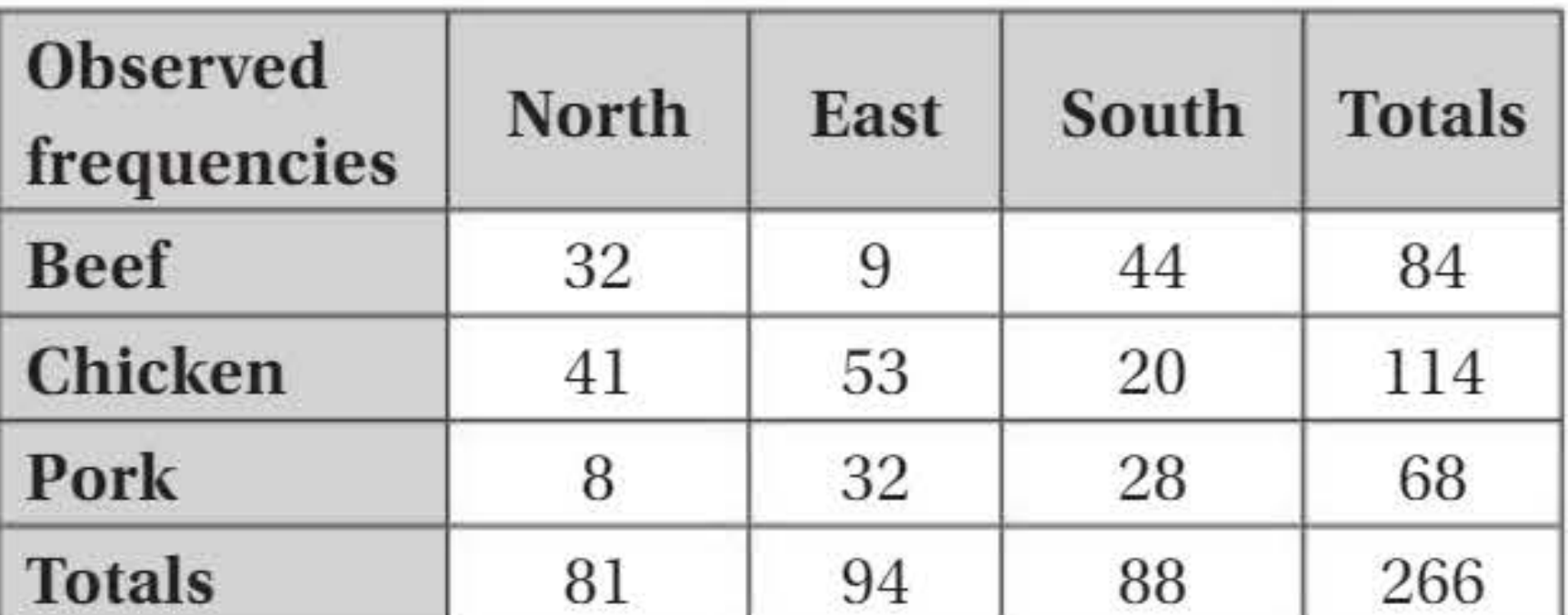
A sample of 266 people from the north, east, and south of a city were asked which meat they liked most: beef, chicken, or pork.

Table

Step 1: Calculate expected frequencies

If the variables (region and meat preference) are independent, the expected frequency for each cell is:

$E_i = \frac{\text{row total} \times \text{column total}}{\text{grand total}}$

For example, for north and beef:

$E = \frac{81 \times 84}{266} = 25.6 \text{ (to 3 sf)}$

The complete table of expected frequencies:

Table

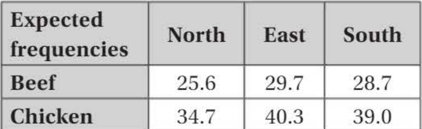
All expected frequencies are above 5, so we can proceed with the test.

Step 2: Set up hypotheses

H₀: There is no association between region and meat preference.

H₁: There is some association between region and meat preference.

Test at the 5% significance level.

Step 3: Calculate X² contributions

For each cell, calculate:

$\frac{(O_i - E_i)^2}{E_i}$

Table

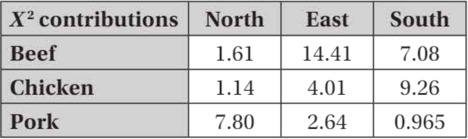
Step 4: Calculate the test statistic

Sum all contributions:

$X^2 = 1.61 + 14.41 + 7.08 + 1.14 + 4.01 + 9.26 + 7.80 + 2.64 + 0.965 = 48.9 \text{ (to 3 sf)}$

Step 5: Determine degrees of freedom

This is a 3×3 table, so:

$\nu = (3-1) \times (3-1) = 4$

Step 6: Find the critical value

From chi-squared tables, $\chi^2_4$ at 5% significance: critical value = 9.49

Step 7: Make a decision

Since $X^2 = 48.9 > 9.49$ , we reject H₀.

Conclusion: There is sufficient evidence at the 5% level to suggest an association between region and meat preference.

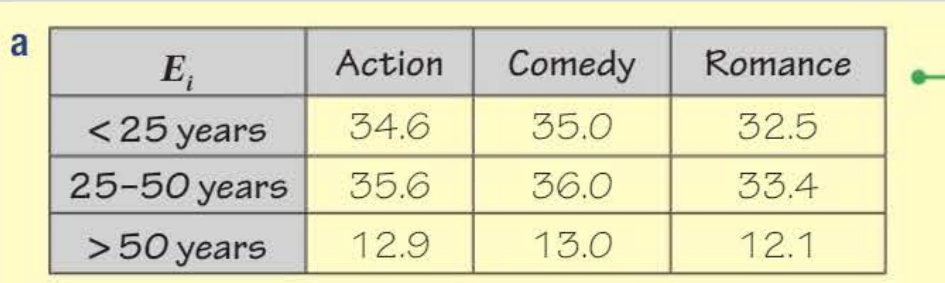
Worked example 2: Movie genre and age

lightbulbExample

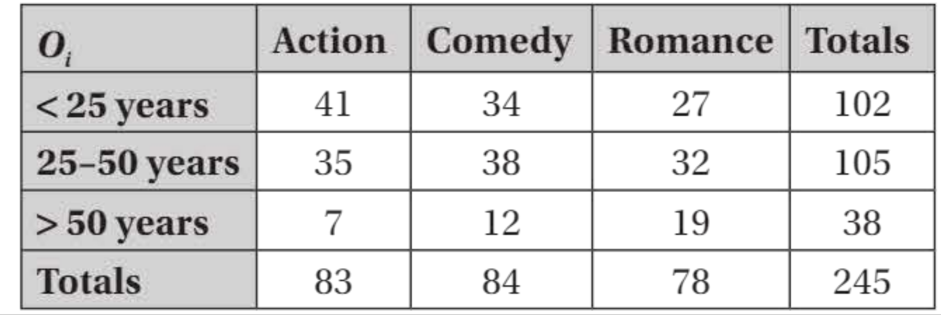
Worked Example: Age and Movie Genre Preferences

A test examines whether there is association between age and movie genre preferences.

Table

Calculate expected frequencies

For the cell corresponding to Action and under 25 years:

$E = \frac{83 \times 102}{245} = 34.6 \text{ (to 3 sf)}$

Complete expected frequency table:

Table

Calculate X² contributions

Table

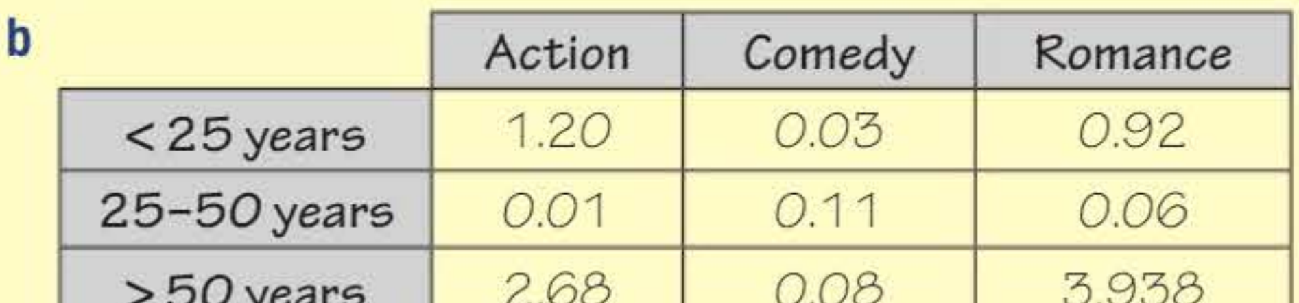
Calculate the test statistic

Total: $X^2 = 9.03$ (to 3 sf)

Degrees of freedom

This is a 3×3 table: $\nu = (3-1) \times (3-1) = 4$

p-value approach

The p-value is P(X ≥ 9.03) = 0.06 where X follows $\chi^2_4$ distribution.

Conclusion

Since the p-value (0.06) is larger than the significance level (0.05), there is insufficient evidence to reject the null hypothesis. We do not have sufficient evidence of an association between age and movie genre preference.

Worked example 3: Voting intentions with grouping

lightbulbExample

Worked Example: Voting Intentions Requiring Category Grouping

Voters in three constituencies were polled about their voting intentions for the Red, Green, and Blue parties.

Table

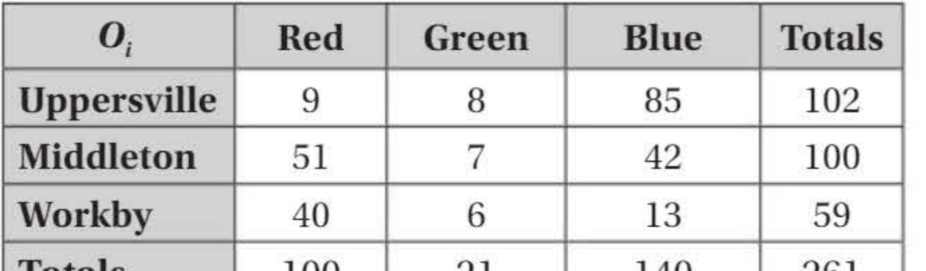
Problem identified: The expected frequency for Green voters in Workby is below 5.

Solution: Group Red and Green together (they have similar policies).

After grouping:

O_i	Red and Green	Blue	Totals
Uppersville	17	85	102
Middleton	58	42	100
Workby	46	13	59
Totals	121	140	261

Calculate expected frequencies

The grouped table now has all expected frequencies above 5.

Degrees of freedom

After grouping: $(3-1) \times (2-1) = 2$ degrees of freedom

After calculating: $X^2 = 65.3$

Critical value at 5% with 2 df: 5.99

Conclusion

Since $X^2 = 65.3 > 5.99$ , there is sufficient evidence to suggest association between location and voting intention.

Important note: Having grouped the data, our conclusion must treat Red and Green intentions together. We cannot make separate claims about Red or Green party support individually.

Worked example 4: Lunch choices (2×2 table with Yates' correction)

lightbulbExample

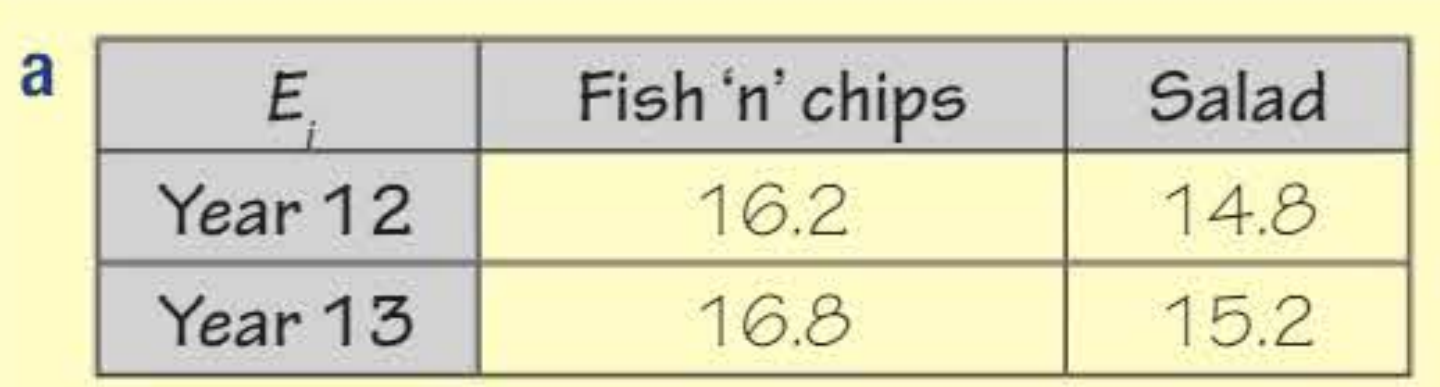
Worked Example: 2×2 Table with Yates' Correction

Year 12 and Year 13 students were asked whether they prefer fish 'n' chips or salad.

Table

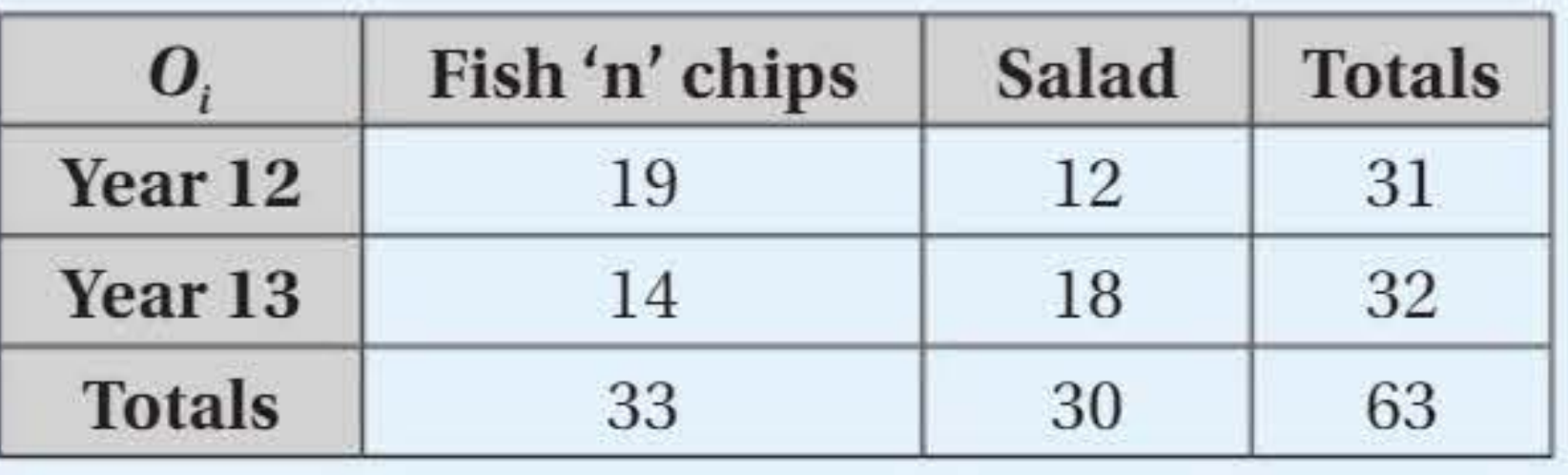
Calculate expected frequencies

Table

Apply Yates' correction

Since this is a 2×2 table, use:

$X^2_{\text{Yates}} = \sum \frac{(|O_i - E_i| - 0.5)^2}{E_i}$

The X² contributions become:

	Fish 'n' chips	Salad
Year 12	0.32	0.35
Year 13	0.31	0.34

Calculate the test statistic

$X^2 = 1.30$ (to 3 sf)

Degrees of freedom

For a 2×2 table: $\nu = 1$

Critical value

At 10% significance with 1 df: critical value = 2.71

Conclusion

Since $X^2 = 1.30 < 2.71$ , there is insufficient evidence to reject the null hypothesis.

There is insufficient evidence of association between year group and lunch choice.

Worked example 5: Height and legroom opinions

lightbulbExample

Worked Example: Height and Legroom Opinions

An airline surveyed passengers of various heights about their opinions on the amount of legroom.

O_i	>1.80m	<1.50m	Between 1.50m and 1.80m	Totals
Too little	67	32	304	403
Too much	19	48	415	482
About right	48	51	379	478
Totals	134	131	1098	1363

Key observations:

The large contributions from people over 1.80m show that their opinions differ most from what is expected.

Looking at observed versus expected frequencies:

There is evidence for a strong positive association between being tall and believing there is too little legroom
There is a strong negative association between being tall and believing there is too much legroom
Short people's opinions about "too much" legroom are very close to expected values

X² statistic: 41.0 (to 3 sf)

Degrees of freedom: $(3-1) \times (3-1) = 4$

Critical value: At 5% significance with 4 df: 9.49

Conclusion

Since $X^2 = 41.0 > 9.49$ , there is sufficient evidence to reject the null hypothesis.

There is sufficient evidence to suggest an association between height and opinions on legroom.

Exam tips

chatImportant

Common Exam Traps to Avoid:

Forgetting to check expected frequencies are ≥ 5 - this is a validity condition that must be verified
Using Yates' correction on tables larger than 2×2 - remember "Yates for 2-by-2" only!
Calculating degrees of freedom incorrectly - always use $(m-1) \times (n-1)$
Not grouping categories when expected frequencies are too low
Stating conclusions about positive/negative association - you only test for presence of association
Forgetting to acknowledge grouped categories in conclusions

infoNote

Problem-Solving Strategy:

Always construct the expected frequency table first
Show your calculation for at least one expected frequency - this demonstrates understanding
Create a table of X² contributions to avoid arithmetic errors
Double-check your degrees of freedom calculation
State your hypotheses clearly before beginning calculations
Write conclusions in context, referencing the original variables

infoNote

Step-by-Step Exam Approach:

Write out hypotheses H₀ and H₁
Calculate and present expected frequencies table
Check all expected frequencies ≥ 5 (group if necessary)
Calculate X² statistic with working
State degrees of freedom with calculation
State critical value or p-value
Make comparison and decision
Write conclusion in context

Remember!

bookmarkSummary

Key Points to Remember:

Contingency tables display the relationship between two categorical variables, showing observed frequencies for each combination of categories.
Expected frequencies are calculated assuming independence: $E_i = \frac{\text{row total} \times \text{column total}}{\text{grand total}}$ , and must all be at least 5 for the test to be valid.
The chi-squared test statistic is $X^2 = \sum \frac{(O_i - E_i)^2}{E_i}$ , which measures how much observed data deviates from expected values under independence.
Degrees of freedom for an $m \times n$ table are $(m-1) \times (n-1)$ , and for 2×2 tables only, apply Yates' correction: $X^2_{\text{Yates}} = \sum \frac{(|O_i - E_i| - 0.5)^2}{E_i}$ .
When any expected frequency is below 5, group similar categories together, recalculate expected frequencies, and adjust degrees of freedom accordingly before conducting the test.

Memory Aids:

"Five alive" - expected frequencies must be at least 5
"Yates for 2-by-2" - only use correction for 2×2 tables
"Rows minus one, columns minus one, multiply done" - degrees of freedom formula
"O-E-D" process - Observe, Expect, Decide

Contingency Tables (AQA A-Level Further Maths): Revision Notes