Continuous Distributions 2 Revision Notes for AQA A-Level Further Maths

Continuous Distributions 2

Introduction to continuous distributions

When working with continuous random variables, we need to understand how to calculate probabilities and find key statistical measures. Unlike discrete variables, continuous variables require integration to find probabilities over intervals.

infoNote

For continuous random variables, we cannot calculate the probability of a single exact value (which is always zero). Instead, we focus on probabilities over intervals using integration.

For a continuous random variable $X$ with probability density function $f(x)$ , the probability that $X$ lies between two values $a$ and $b$ is:

$P(a < X < b) = \int_a^b f(x)\,dx$

The mean (expected value) and variance of $X$ are given by:

$\mu = E(X) = \int_{-\infty}^{\infty} xf(x)\,dx$

$\sigma^2 = \text{Var}(X) = E[X^2] - \mu^2 = \int_{-\infty}^{\infty} x^2f(x)\,dx - \mu^2$

These formulas extend the concepts you learned for discrete distributions to the continuous case.

The cumulative distribution function

Definition

The cumulative distribution function (CDF), denoted $F(x)$ , is a powerful tool for calculating probabilities and finding percentiles. It tells you the probability that a random variable takes a value less than or equal to a particular value.

Key definition: For a continuous random variable $X$ , the CDF is defined as:

$F(x) = P(X < x) = P(X \leq x)$

chatImportant

For continuous distributions, $P(X = x) = 0$ , so $P(X < x) = P(X \leq x)$ . This is different from discrete distributions where the probability at a specific point can be non-zero.

Calculating the CDF from the PDF

Since $F(x)$ represents the probability up to value $x$ , we can calculate it by integrating the probability density function from $-\infty$ to $x$ :

$F(x) = \int_{-\infty}^{x} f(t)\,dt$

This integral accumulates all the probability from the lowest possible value up to $x$ .

infoNote

Properties of the CDF:

$F(x)$ is always non-decreasing
$\lim_{x \to -\infty} F(x) = 0$ and $\lim_{x \to \infty} F(x) = 1$
$F(x)$ is continuous for continuous random variables

Finding the PDF from the CDF

The relationship between the PDF and CDF works both ways. If you know the CDF, you can find the PDF by differentiation:

$f(x) = \frac{d}{dx}F(x)$

This relationship comes from the fundamental theorem of calculus. It means the PDF is the rate of change of the CDF.

chatImportant

Verification Check: Always check that your PDF integrates to 1 over its entire domain. This is a quick way to verify your answer is correct and catch potential errors early.

Finding parameters using normalization

The total probability for any random variable must equal 1. This principle is called normalization and is used to find unknown parameters in probability density functions.

If $f(x)$ is a valid PDF, then:

$\int_{-\infty}^{\infty} f(x)\,dx = 1$

For a PDF defined on a finite interval $[a, b]$ :

$\int_a^b f(x)\,dx = 1$

lightbulbExample

Worked Example 1: Finding parameter values

A continuous random variable $X$ has probability density function:

$f(x) = \begin{cases} 4x^a & 0 \leq x \leq 1 \\ 0 & \text{otherwise} \end{cases}$

Part a: Find the value of $a$ .

Solution:

Using the normalization condition:

$\int_0^1 4x^a\,dx = 1$

$\left[\frac{4x^{a+1}}{a+1}\right]_0^1 = 1$

$\frac{4}{a+1} = 1$

$a + 1 = 4$

$\therefore a = 3$

Therefore, $f(x) = 4x^3$ for $0 \leq x \leq 1$ .

Part b: Find the cumulative distribution function $F(x)$ .

Solution:

For $0 \leq x \leq 1$ :

$F(x) = \int_0^x 4t^3\,dt = \left[t^4\right]_0^x = x^4$

The complete CDF is:

$F(x) = \begin{cases} 0 & x < 0 \\ x^4 & 0 \leq x \leq 1 \\ 1 & x > 1 \end{cases}$

Part c: Find the median value $M$ of $X$ .

Solution:

The median is the value where $F(M) = 0.5$ or equivalently where $\int_0^M f(x)\,dx = 0.5$ .

$\int_0^M 4x^3\,dx = \frac{1}{2}$

$M^4 = \frac{1}{2}$

$M = \left(\frac{1}{2}\right)^{1/4} = 0.841 \text{ (3 dp)}$

Working with exponential-type distributions

Exponential distributions are commonly used to model waiting times, lifetimes, and decay processes. The exponential CDF has the characteristic form $F(x) = 1 - e^{-\lambda x}$ for $x \geq 0$ , where $\lambda$ is a positive parameter.

lightbulbExample

Worked Example 2: Exponential CDF

A random variable $X$ has cumulative distribution function $F(x) = 1 - e^{-\lambda x}$ for $x \geq 0$ .

Part a: Find the probability density function of $X$ .

Solution:

Using the relationship $f(x) = \frac{d}{dx}F(x)$ :

$f(x) = \frac{d}{dx}(1 - e^{-\lambda x}) = \frac{d}{dx}(1) - \frac{d}{dx}(e^{-\lambda x})$

$f(x) = 0 - (-\lambda e^{-\lambda x}) = \lambda e^{-\lambda x}$

Chain Rule Reminder: When differentiating exponential functions, remember the chain rule. The derivative of $e^{-\lambda x}$ is $-\lambda e^{-\lambda x}$ (multiply by the derivative of the exponent).

Part b: Write the modal value of $X$ .

Solution:

The mode is the value where $f(x)$ is maximum. For $f(x) = \lambda e^{-\lambda x}$ , this occurs when $x = 0$ (the exponential function decreases as $x$ increases).

Mode = 0

Part c: Prove that when two $X$ values are chosen at random, the probability that one is less than $x_1$ and the other is more than $x_1$ is $2e^{-\lambda x_1}(1 - e^{-\lambda x_1})$ .

Solution:

This is a problem about two independent outcomes:

Probability first value less than $x_1$ : $F(x_1) = 1 - e^{-\lambda x_1}$
Probability second value more than $x_1$ : $P(X > x_1) = 1 - F(x_1) = e^{-\lambda x_1}$

The outcome can occur in two ways (first less and second more, OR first more and second less):

$P = 2 \times P(X < x_1) \times P(X > x_1)$

$P = 2(1 - e^{-\lambda x_1})(e^{-\lambda x_1}) = 2e^{-\lambda x_1}(1 - e^{-\lambda x_1})$ :::

Piecewise probability density functions

Some PDFs are defined differently over different intervals. These require careful integration, with separate calculations for each piece.

chatImportant

When working with piecewise functions, always:

Integrate each piece separately over its specified interval
Add the results from all pieces when calculating total probability
Remember to include contributions from earlier intervals when building the CDF

lightbulbExample

Worked Example 3: Piecewise PDF

A continuous random variable $X$ has probability density function:

$f(x) = \begin{cases} ax^2 & 0 < x \leq 1 \\ \frac{-9x + 15}{4} & 1 < x < \frac{5}{3} \\ 0 & \text{otherwise} \end{cases}$

Part a: Show that $a = \frac{3}{2}$ .

Solution:

Using normalization over the entire domain:

$\int_0^1 ax^2\,dx + \int_1^{5/3} \frac{-9x + 15}{4}\,dx = 1$

First integral:

$\int_0^1 ax^2\,dx = \left[\frac{ax^3}{3}\right]_0^1 = \frac{a}{3}$

Second integral:

$\int_1^{5/3} \frac{-9x + 15}{4}\,dx = \frac{1}{4}\left[\frac{-9x^2}{2} + 15x\right]_1^{5/3}$

$= \frac{1}{4}\left[\left(\frac{-9(5/3)^2}{2} + 15 \times \frac{5}{3}\right) - \left(\frac{-9}{2} + 15\right)\right]$

$= \frac{1}{4}\left[\frac{-25}{2} + 25 - \frac{-9}{2} - 15\right] = \frac{1}{4}\left[\frac{-16}{2} + 10\right] = \frac{1}{2}$

Therefore:

$\frac{a}{3} + \frac{1}{2} = 1 \implies \frac{a}{3} = \frac{1}{2} \implies a = \frac{3}{2}$

Part b: Find the cumulative distribution function $F(x)$ .

Solution:

We need to integrate the PDF in pieces:

For $0 < x \leq 1$ :

$F(x) = \int_0^x \frac{3t^2}{2}\,dt = \left[\frac{t^3}{2}\right]_0^x = \frac{x^3}{2}$

For $1 < x < \frac{5}{3}$ :

$F(x) = \int_0^1 \frac{3t^2}{2}\,dt + \int_1^x \frac{-9t + 15}{4}\,dt$

$= \frac{1}{2} + \frac{1}{4}\left[\frac{-9t^2}{2} + 15t\right]_1^x$

$= \frac{1}{2} + \frac{1}{4}\left[\frac{-9x^2}{2} + 15x - \frac{-9}{2} - 15\right]$

$= \frac{-9x^2}{8} + \frac{15x}{4} + \frac{17}{8}$

The complete CDF is:

$F(x) = \begin{cases} 0 & x \leq 0 \\ \frac{x^3}{2} & 0 < x \leq 1 \\ \frac{-9x^2}{8} + \frac{15x}{4} + \frac{17}{8} & 1 < x < \frac{5}{3} \\ 1 & x \geq \frac{5}{3} \end{cases}$

Part c: Find the median and interquartile range of $X$ .

Solution:

The median satisfies $F(M) = 0.5$ . Since $F(1) = 0.5$ , the median is M = 1.

For quartiles, we need $F(Q_1) = 0.25$ and $F(Q_3) = 0.75$ .

For $Q_1$ (in the first interval):

$\frac{Q_1^3}{2} = \frac{1}{4}$

$Q_1^3 = \frac{1}{2}$

$Q_1 = \sqrt[3]{\frac{1}{2}} = 0.79 \text{ (2 dp)}$

For $Q_3$ (in the second interval):

$\frac{-9Q_3^2}{8} + \frac{15Q_3}{4} + \frac{17}{8} = \frac{3}{4}$

Solving this quadratic equation gives $Q_3 = 1.20$ (2 dp).

The interquartile range is:

$\text{IQR} = Q_3 - Q_1 = 1.20 - 0.79 = 0.41$

The rectangular (uniform) distribution

The rectangular distribution (also called the uniform distribution) is one of the simplest continuous distributions. It models situations where all values in an interval are equally likely to occur.

Definition and properties

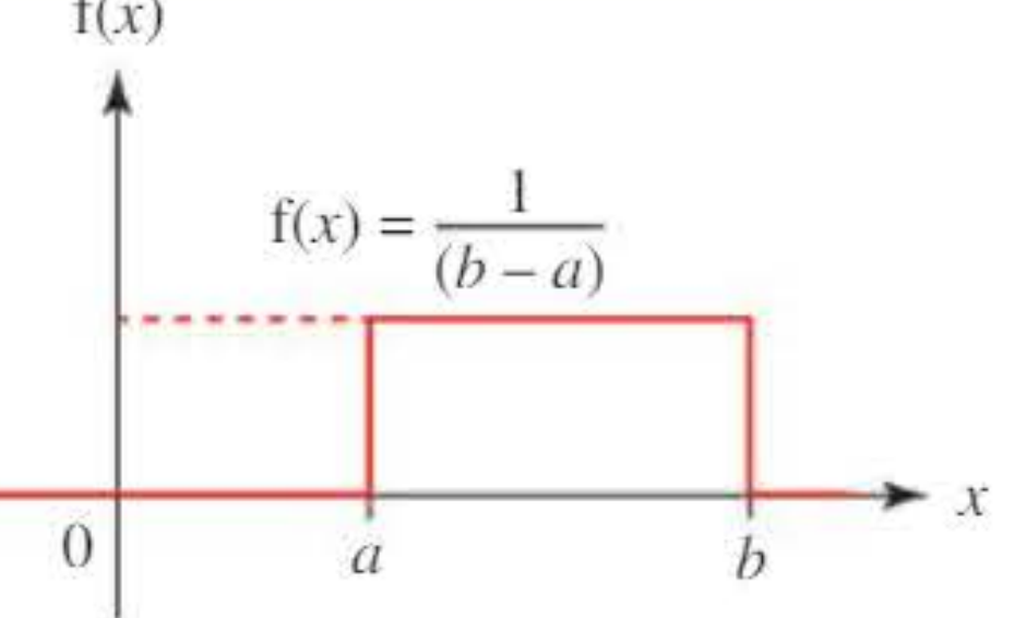
Definition: A random variable $R$ follows a rectangular distribution on the interval $(a, b)$ if all values in this interval are equally likely. We write $R \sim \text{Rectangular}(a, b)$ .

The probability density function is constant over the interval:

$f(r) = \begin{cases} \frac{1}{b-a} & a < r < b \\ 0 & \text{otherwise} \end{cases}$

infoNote

The constant $\frac{1}{b-a}$ ensures that the total area under the PDF equals 1. Since the PDF forms a rectangle of width $(b-a)$ and height $\frac{1}{b-a}$ , the area is $(b-a) \times \frac{1}{b-a} = 1$ .

Mean of rectangular distribution

The mean (expected value) of a rectangularly distributed random variable is:

$E(R) = \int_a^b r \cdot \frac{1}{b-a}\,dr = \frac{1}{b-a} \int_a^b r\,dr$

$= \frac{1}{b-a} \left[\frac{r^2}{2}\right]_a^b = \frac{1}{b-a} \times \frac{b^2 - a^2}{2}$

$= \frac{(b-a)(b+a)}{2(b-a)} = \frac{a+b}{2}$

This makes intuitive sense: the mean is the midpoint of the interval.

Variance of rectangular distribution

The variance requires calculating $E(R^2)$ first:

$E(R^2) = \int_a^b r^2 \cdot \frac{1}{b-a}\,dr = \frac{1}{b-a}\left[\frac{r^3}{3}\right]_a^b = \frac{b^3 - a^3}{3(b-a)}$

Using the factorisation $b^3 - a^3 = (b-a)(b^2 + ab + a^2)$ :

$E(R^2) = \frac{b^2 + ab + a^2}{3}$

Then:

$\text{Var}(R) = E(R^2) - [E(R)]^2 = \frac{b^2 + ab + a^2}{3} - \left(\frac{a+b}{2}\right)^2$

After algebraic manipulation (expanding and simplifying):

$\text{Var}(R) = \frac{(b-a)^2}{12}$

chatImportant

Key formulas for rectangular distribution:

$E(R) = \frac{a+b}{2} \quad \text{and} \quad \text{Var}(R) = \frac{(b-a)^2}{12}$

These formulas are essential for working with uniform distributions efficiently. Remember them!

lightbulbExample

Worked Example 4: Measurement error

The length of a line segment is measured to the nearest millimetre. Calculate the mean and variance of the error in any recorded length.

Solution:

Let $X$ be the error (in mm) in the recorded length. The error can be anywhere from $-0.5$ mm to $+0.5$ mm, with all values equally likely:

$X \sim \text{Rectangular}(-0.5, 0.5)$

Here $a = -0.5$ and $b = 0.5$ .

Mean:

$E(X) = \frac{a+b}{2} = \frac{-0.5 + 0.5}{2} = 0$

This makes sense: on average, the error is zero (measurements are equally likely to be too high or too low).

Variance:

$\text{Var}(X) = \frac{(b-a)^2}{12} = \frac{(0.5-(-0.5))^2}{12} = \frac{1}{12}$

Rounding Error Tip: Rounding errors typically follow a rectangular distribution with range equal to the rounding interval. For "nearest millimetre", the range is 1 mm, giving variance $\frac{1}{12}$ . For "nearest centimetre", it would be $\frac{1^2}{12} = \frac{1}{12}$ cm², and so on.

:::

Mixed distributions

Some random variables are partly discrete and partly continuous. For example, queuing times may be exactly zero with some probability (discrete), or take positive continuous values.

chatImportant

When working with mixed distributions:

Calculate the discrete probabilities separately
Integrate the continuous PDF over its domain
Ensure the sum of all discrete probabilities plus the integral of the continuous PDF equals 1
For expectations, add the discrete contribution (value × probability) to the continuous contribution (integral)

lightbulbExample

Worked Example 5: Supermarket waiting times

Supermarket checkout waiting times, $T$ minutes, have the following distribution:

$P(T = 0) = c, \quad f(t) = k(t-3) \text{ for } 0 < t \leq 3$

Part a: Prove that $k = \frac{2(c-1)}{9}$ .

Solution:

The total probability must equal 1. This includes the discrete part and the continuous part:

$P(T=0) + \int_0^3 k(t-3)\,dt = 1$

$c + k\int_0^3 (t-3)\,dt = 1$

Evaluating the integral:

$\int_0^3 (t-3)\,dt = \left[\frac{t^2}{2} - 3t\right]_0^3 = \left(\frac{9}{2} - 9\right) - 0 = -\frac{9}{2}$

Therefore:

$c + k\left(-\frac{9}{2}\right) = 1$

$c - \frac{9k}{2} = 1$

$\frac{9k}{2} = c - 1$

$k = \frac{2(c-1)}{9}$

Part b: If the probability of zero waiting time is 0.4, show that the expected waiting time is 54 seconds and find the probability that the waiting time exceeds one minute.

Solution:

Given $c = 0.4$ :

$k = \frac{2(0.4-1)}{9} = \frac{2(-0.6)}{9} = -\frac{2}{15}$

Expected waiting time:

$E(T) = 0 \times 0.4 + \int_0^3 t \times \left(-\frac{2}{15}\right)(t-3)\,dt$

$= -\frac{2}{15}\int_0^3 (t^2 - 3t)\,dt$

$= -\frac{2}{15}\left[\frac{t^3}{3} - \frac{3t^2}{2}\right]_0^3$

$= -\frac{2}{15}\left(9 - \frac{27}{2}\right) = -\frac{2}{15} \times \left(-\frac{9}{2}\right) = \frac{9}{10}$

So $E(T) = 0.9$ minutes $= 54$ seconds.

Probability waiting time exceeds 1 minute:

$P(T > 1) = \int_1^3 \left(-\frac{2}{15}\right)(t-3)\,dt$

$= -\frac{2}{15}\left[\frac{t^2}{2} - 3t\right]_1^3$

$= -\frac{2}{15}\left[\left(\frac{9}{2} - 9\right) - \left(\frac{1}{2} - 3\right)\right]$

$= -\frac{2}{15}\left[-\frac{9}{2} + \frac{5}{2}\right] = -\frac{2}{15} \times (-2) = \frac{4}{9}$

bookmarkSummary

Problem-solving strategy

When working with continuous distributions:

1. Integrate the PDF to find probabilities and the cumulative distribution function. Remember that probabilities are areas under the curve.

2. Recognise rectangular distributions and use the formulas $E(R) = \frac{a+b}{2}$ and $\text{Var}(R) = \frac{(b-a)^2}{12}$ when appropriate.

3. Calculate mean and variance using the standard formulas with integration. For rectangular distributions, use the shortcut formulas.

4. Handle mixed distributions carefully, treating discrete and continuous parts separately. The total probability is the sum of discrete probabilities plus the integral of the continuous PDF.

Exam tips:

Always check your PDF integrates to 1 (accounting for any discrete probabilities)
When finding the CDF, remember to include constant terms from earlier intervals
For the median, solve $F(M) = 0.5$
Sketch the PDF when possible to visualise the distribution
Watch for negative signs in exponential distributions when differentiating

bookmarkSummary

Remember!

Key Concepts:

The cumulative distribution function $F(x) = P(X < x) = \int_{-\infty}^{x} f(t)\,dt$ gives the probability up to any value.
The PDF and CDF are related by differentiation: $f(x) = \frac{d}{dx}F(x)$ , and integration works the other way.
For the rectangular distribution $R \sim \text{Rectangular}(a,b)$ : the PDF is $f(r) = \frac{1}{b-a}$ , the mean is $E(R) = \frac{a+b}{2}$ , and the variance is $\text{Var}(R) = \frac{(b-a)^2}{12}$ .
Always use the normalization condition $\int f(x)\,dx = 1$ to find unknown parameters in a PDF.
Mixed distributions require treating discrete and continuous parts separately, ensuring total probability equals 1.

Continuous Distributions 2 (AQA A-Level Further Maths): Revision Notes