Goodness of Fit (Edexcel A-Level Further Mathematics): Revision Notes
21.2.1 Goodness of Fit
Goodness of Fit Tests
The test can be used to test how well a distribution fits a data set.
Example: Eggs are sold in four categories: small, medium, large, and extra large. A supermarket model predicts that these will be sold in the ratio 1:2:3:1. To check this model, the supermarket looks at sales in a store in one day.
| Size of eggs | Small | Medium | Large | Extra large |
|---|---|---|---|---|
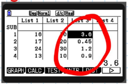
| Number sold | 16 | 17 | 24 | 13 |
Use an appropriate statistical test to determine if the model fits this data, using a 5% significance level.
1. State hypotheses
- : Eggs are sold in the ratio .
- : Eggs are not sold in the ratio .
2. Calculate expectations by splitting total into the given ratio
- Total
- in the ratio
- → | Size of eggs | Small | Medium | Large | Extra large | |---|---|---|---|---| | Number sold | 16 | 17 | 24 | 13 | | Expected | 10 | 20 | 30 | 10 |
3. Perform a test on the differences. Note that for goodness of fit tests, even when , a Yates correction is never required.
Contributions:
- See calculator screenshot for instructions.
Goodness of Fit on Graphical Calculator
Steps:
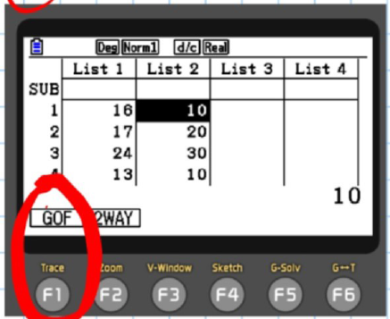
A) Go to Tests on the calculator and choose χ² GOF (Goodness of Fit).

B) Input observed and expected data in the respective lists (List 1, List 2).
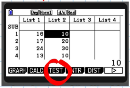
C) After inputting the data, choose χ² GOF test.
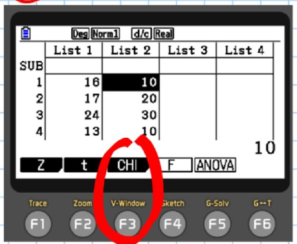
D) Select List1 for observed values and List2 for expected values.
E) Input degrees of freedom ().
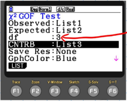
In this case, v = 3 because there are four categories (), and the total has only one constraint, so degrees of freedom .
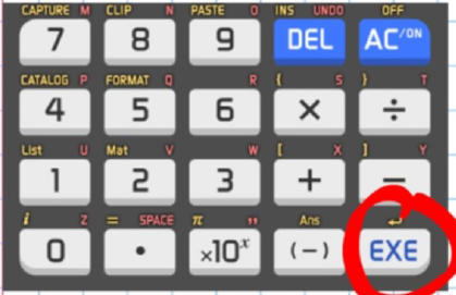
F) Execute the test by pressing EXE.
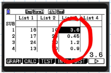
G) The calculator will display and .
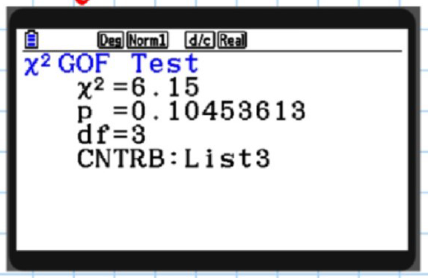
H) and are shown.
I) Pressing Exit twice provides detailed results, including contributions in List 3.
4. Conclusion:
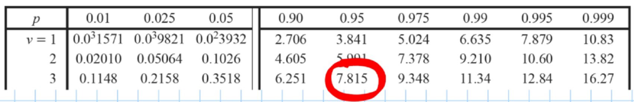
Since χ²calc = 6.15 < 7.815, we do not reject .
Insufficient evidence to suggest that the ratio of eggs sold differs from the ratio 1:2:3:1.
Testing Hypothesis of Fit for Any Distribution
It is possible to test whether any known model fits a set of data.
Note: The model fits the data, not the data fits the model.
Past Paper Example
Q4, (Jan 2008, Q4a)
In Germany, towards the end of the nineteenth century, a study was undertaken into the distribution of the sexes in families of various sizes. The table shows some data about the number of girls in 500 families, each with 5 children. It is thought that the binomial distribution B(5, p) should model these data.
| Number of girls | Number of families |
|---|---|
| 0 | 32 |
| 1 | 110 |
| 2 | 154 |
| 3 | 125 |
| 4 | 63 |
| 5 | 16 |
i) Use this information to calculate an estimate for the mean number of girls per family of 5 children. Hence show that 0.45 can be taken as an estimate of p.
ii) Investigate at a 5% significance level whether the binomial model with p estimated as 0.45 fits the data. Comment on your findings and also on the extent to which the conditions for a binomial model are likely to be met. [12 marks]
Solution: i)
Since we have estimated one of the population parameters, this means we have one less degree of freedom. Remember this point when checking critical values from the table.
Solution: ii)
Step 1: State hypotheses:
- : The proposed model fits the data well.
- : The proposed model does not fit the data well.
Step 2: Using the proposed model: Calculate the proportion of the total frequency associated with each outcome.
Using :
Now, dividing the total frequency with the proportions, we get expectations:
Expectations:
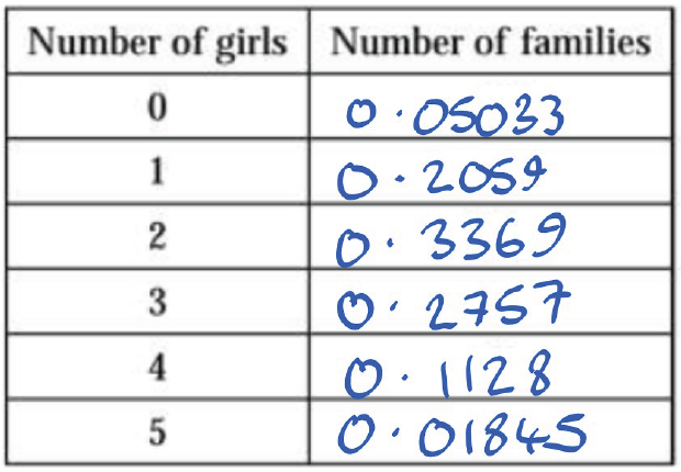
| Number of girls | Number of families | | |---|---|---|---| | 0 | 25.165 | | | 1 | 102.95 | | | 2 | 168.45 | | | 3 | 137.85 | | | 4 | 56.4 | | | 5 | 9.225 | |
Notice no expectations < 5 no combining of items.
Observations:
| Number of girls | Number of families |
|---|---|
| 0 | 32 |
| 1 | 110 |
| 2 | 154 |
| 3 | 125 |
| 4 | 63 |
| 5 | 16 |
Step 3: Calculate where contributions are calculated by:
Note: If asked to analyse contributions, it is necessary to calculate the value of each individual contribution.
Step 4: Check the critical value and conclude appropriately.
- Remember:
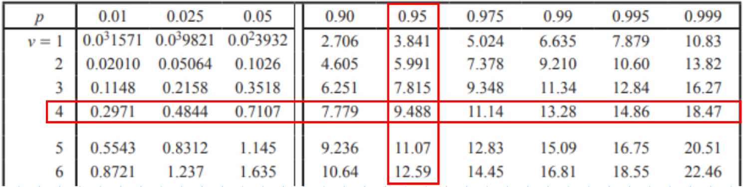
Critical Value (C.V.) from the table:
Calculated value:
Conclusion: Reject H₀.
The binomial model is not a good fit for the data.
In the proposed model, we seem to underestimate in the extremes and overestimate in the middle.
The biggest contribution is for , indicating that this model is a poor fit, especially at the right-hand tail.
Within a family, the sex of one child may not be statistically independent of a previously born child. Also, the probability of giving birth to a girl is unlikely to be across all families. Therefore, the binomial model may not be appropriate.