Equipment Replacement and Maintenance (Leaving Cert Applied Maths): Revision Notes
Equipment Replacement and Maintenance
Equipment replacement and maintenance is a critical business decision that can be optimised using dynamic programming techniques. This approach helps determine the most cost-effective timing for replacing equipment such as vehicles, machinery, or other assets.
Understanding the problem
In equipment replacement problems, we need to decide when to replace an asset to minimise the total cost over a given time period. The key challenge is balancing the increasing maintenance costs of older equipment against the high initial cost of new equipment.
The timing of equipment replacement creates a fundamental trade-off: keeping equipment too long results in high maintenance costs, while replacing it too frequently results in high purchase costs and lost resale value.
Key components of the cost calculation:
- Purchase cost - the initial cost of buying new equipment
- Maintenance cost - ongoing costs that typically increase with age
- Resale value - the amount recovered when selling the equipment
- Future optimal value - the minimum cost from that point onwards
The cost formula
The total cost for any decision is calculated using:
This formula considers both immediate costs and the optimal decisions that will be made in future years. Understanding this relationship is crucial for solving equipment replacement problems correctly.
Dynamic programming approach
Dynamic programming solves this problem by working backwards from the final year. This backwards induction method ensures we always know the optimal future value when making current decisions.
The backwards approach is essential because we need to know the optimal future costs before we can determine the best current decision. This distinguishes dynamic programming from other optimisation methods.
Setting up the decision table
The solution uses a structured table with these columns:
- Stage (Year) - the time period we're analysing
- State - number of years left when purchasing equipment
- Action - decision about how long to keep the equipment
- Destination - years remaining when we sell the equipment
- Value - total cost of this decision path
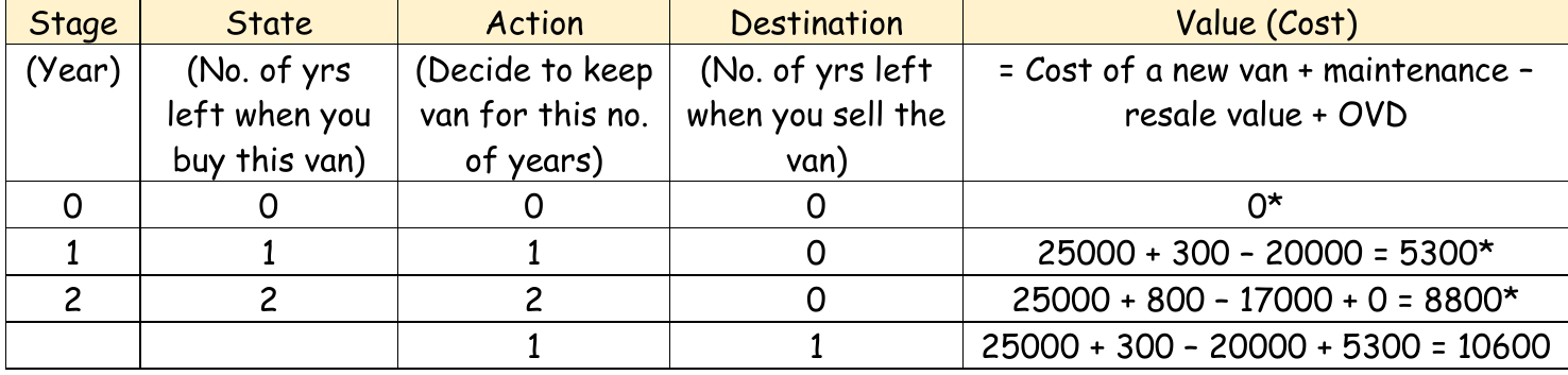
This initial table shows how we begin the analysis, starting with the final years and working backwards.
Working through the solution
Worked Example: The Backwards Solution Process
Step 1: Start with the final stages Begin by analysing the last few years of the planning period. At the very end (year 0), no action is needed, so the cost is zero.
Step 2: Build backwards systematically For each earlier year, calculate the cost of each possible action (keeping the equipment for 1, 2, or 3 years). The action with the lowest total cost becomes the optimal choice, marked with an asterisk (*).
Step 3: Complete the full analysis Continue this process until you reach the beginning of the planning period.
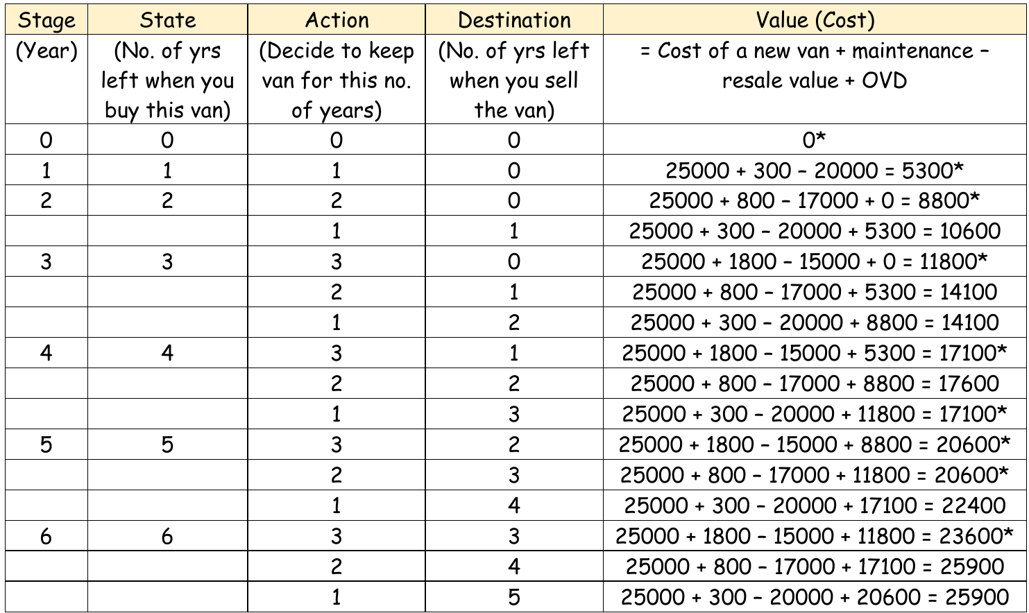
The complete table shows all possible decisions across the entire planning period. Optimal decisions at each stage are marked with asterisks.
Finding the optimal solution
To find the best overall strategy:
- Identify optimal actions - look for entries marked with asterisks (*)
- Follow the optimal path - trace the sequence of optimal decisions
- Interpret the results - understand what the solution means in practical terms
In this example, the optimal strategy is to replace the equipment after 3 years and continue this pattern throughout the planning period.
Practical considerations
When applying this method:
- Maintenance costs typically increase as equipment ages due to wear and tear
- Resale values decrease over time as equipment depreciates
- The planning horizon should be long enough to capture the full replacement cycle
- All costs should be in present value terms for accurate comparison
Common Mistake to Avoid: Don't forget to convert all future costs to present value terms. Failing to account for the time value of money will lead to incorrect replacement decisions.
Exam tips
Essential Exam Strategies:
- Always work backwards from the final year
- Mark optimal decisions clearly with asterisks
- Double-check your cost calculations using the formula
- Remember that the optimal path follows the asterisked entries
- Show your working clearly in tabular form
Key Points to Remember:
- Dynamic programming works backwards - start from the end and work towards the beginning
- The cost formula includes four components - purchase cost, maintenance, resale value, and future optimal value
- Optimal decisions are marked with asterisks (*) in the decision table
- Follow the asterisked path to find the complete optimal replacement strategy
- Maintenance costs increase and resale values decrease over time, creating the trade-off that makes timing crucial