Time-Velocity Graphs Revision Notes for Leaving Cert Applied Maths

Time-Velocity Graphs

What are time-velocity graphs?

Time-velocity graphs are essential tools in kinematics that show how the velocity of an object changes over time. These graphs plot time on the horizontal axis and velocity on the vertical axis. Understanding how to interpret these graphs is crucial for solving motion problems, particularly those involving uniform acceleration.

infoNote

When dealing with motion under constant acceleration, time-velocity graphs typically appear as straight lines. The slope of the line represents the acceleration of the object - a steeper positive slope indicates greater acceleration, while a negative slope shows deceleration.

The fundamental principle: Area equals distance

One of the most important concepts in interpreting time-velocity graphs is understanding what the area under the curve represents. This is a key relationship that you must remember:

chatImportant

The area under a time-velocity graph represents the total distance travelled.

This principle works for all types of motion, whether the graph is linear (constant acceleration) or curved (changing acceleration).

Let's explore why this relationship holds true.

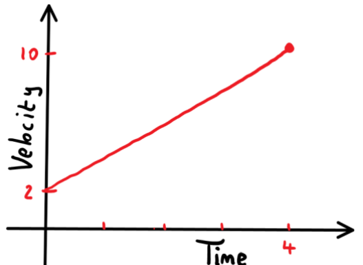
The graph above demonstrates this concept with a simple example showing uniform acceleration from 2 m/s to 10 m/s over 4 seconds, resulting in a total displacement of 40 metres.

Mathematical proof using kinematic equations

To understand why the area under a time-velocity graph gives us distance, we can use the fundamental kinematic equation for uniform acceleration:

$v = u + at$

Where:

$v$ = final velocity
$u$ = initial velocity
$a$ = acceleration
$t$ = time

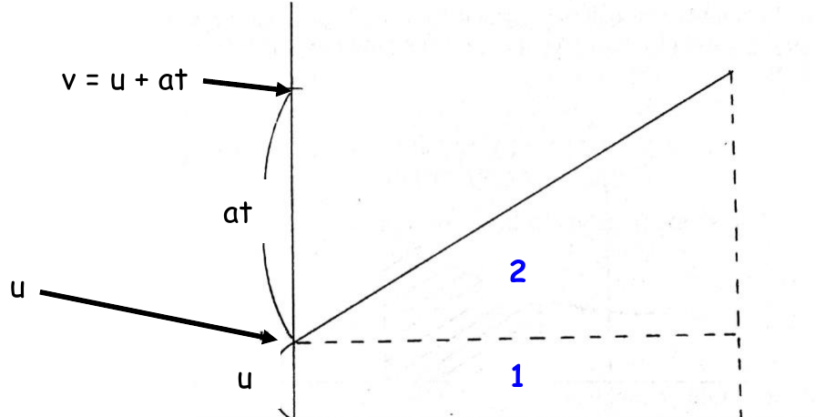
This vector diagram shows how the kinematic equation $v = u + at$ can be visualised geometrically. The diagram demonstrates that final velocity is the vector sum of initial velocity and the change in velocity due to acceleration.

When we plot this relationship on a time-velocity graph, we can calculate the area using basic geometry:

infoNote

Area Under Graph = Area of Rectangle + Area of Triangle

$\text{Area} = ut + \frac{1}{2}(at)(t)$

$\text{Area} = ut + \frac{1}{2}at^2$

This expression is actually the kinematic equation for displacement, proving that the area under the graph indeed represents the distance travelled.

Working with complex motion graphs

Many real-world motion problems involve multiple phases of movement. These might include periods of acceleration, constant velocity, and deceleration. To find the total distance travelled, we break the graph into simpler geometric shapes and calculate each area separately.

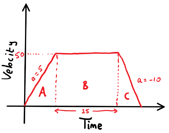
This graph shows a typical three-phase motion scenario with distinct sections labelled A, B, and C.

infoNote

Strategy for Complex Graphs: Break the graph into simpler geometric shapes (triangles and rectangles) and calculate each area separately. Then sum all areas to get the total distance.

Worked example: Car motion analysis

lightbulbExample

Worked Example: Car Motion Analysis

Problem: A car accelerates at 5 m/s² from rest to 50 m/s, then travels at steady speed for 25 seconds, and finally decelerates to rest at 10 m/s².

Solution approach:

Draw the time-velocity graph
Calculate the time for each phase
Find the area of each section
Sum the areas for total distance

Phase calculations:

Section A (acceleration phase):

Using $v = u + at$ : $50 = 0 + 5t$
Therefore: $t = 10$ seconds
Area = $\frac{1}{2} \times \text{base} \times \text{height} = \frac{1}{2} \times 10 \times 50 = 250$ m

Section B (constant velocity phase):

Time = 25 seconds (given)
Area = $\text{base} \times \text{height} = 25 \times 50 = 1250$ m

Section C (deceleration phase):

Using $v = u + at$ : $0 = 50 + (-10)t$
Therefore: $t = 5$ seconds
Area = $\frac{1}{2} \times 5 \times 50 = 125$ m

Total distance = 250 + 1250 + 125 = 1625 m

Average speed = Total distance ÷ Total time = 1625 ÷ (10 + 25 + 5) = 40.625 m/s

Key calculation strategies

When working with time-velocity graphs, remember these essential strategies:

infoNote

Essential Calculation Strategies:

Break complex graphs into simple shapes: Use triangles for acceleration/deceleration phases and rectangles for constant velocity phases
Calculate areas systematically: Work through each section methodically
Check your units: Ensure velocity is in m/s and time in seconds to get distance in metres
Use kinematic equations: Apply $v = u + at$ to find missing time values when needed

For graphs that aren't linear (non-uniform acceleration), more advanced mathematical techniques like integration would be required, but these are beyond the scope of Leaving Certificate Applied Mathematics.

Exam tips

chatImportant

Critical Exam Strategies:

Always start by identifying what type of motion each section of the graph represents
Label your graphs clearly with values and units
Show your working step by step when calculating areas
Remember to include units in your final answers
Double-check that your calculated times and distances make physical sense

Summary

bookmarkSummary

Key Points to Remember:

The area under any time-velocity graph always equals the total distance travelled
Break complex graphs into triangles and rectangles for easier calculation
Use $v = u + at$ to find missing time values in uniform acceleration problems
Average speed = Total distance ÷ Total time for the entire journey
Always check your units and ensure your answers make physical sense

Time-Velocity Graphs (Leaving Cert Applied Maths): Revision Notes