Algorithms (Leaving Cert Computer Science): Revision Notes
Algorithms
Introduction to Algorithms
An algorithm is a finite, well-defined sequence of instructions or steps designed to perform a specific task or solve a particular problem.
Characteristics of Algorithms
Finite : An algorithm must have a finite number of steps. It should terminate after a certain number of steps, producing a result or recognising that no solution exists.
Unambiguous : Each step of an algorithm must be precisely defined and unambiguous. The actions to be performed should be clear and well-understood.
Time Complexity
Time complexity is a measure of the amount of computational time that an algorithm takes to complete as a function of the size of the input.
Time Complexity Example
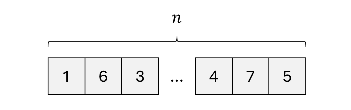
Consider a list of integers. We want to determine the time complexity of performing a linear search to find a specific integer.
The steps for linear search are as follows :
- Start at the beginning of the list.
- Compare the current element with the target value.
- If the current element matches the target value, return the current position of the element.
- If the current element does not match the target value, move to the next element, incrementing the index variable.
- Continue this process until you either find the target value or reach the end of the list.
- In the best case, the target value happens to be the first value in the list. This means we had to make one comparison.
- In the worst case, the target value happens to be the last value in the list or not present at all in the list. This means we had to make comparisons since there are elements.
- In the average case, the target value may lie in the middle of the list which means we had to make comparisons.
Time complexity is always measured in terms of the worst case, which gives an upper bound on the resources required by the algorithm.
Let's take some instances of the linear search algorithm for different sizes of .
| comparisons (worst case) | |
|---|---|
| 1 | 1 |
| 10 | 10 |
| 20 | 20 |
| 30 | 30 |
There is a linear relationship between the size of the input and the maximum number of comparisons needed.
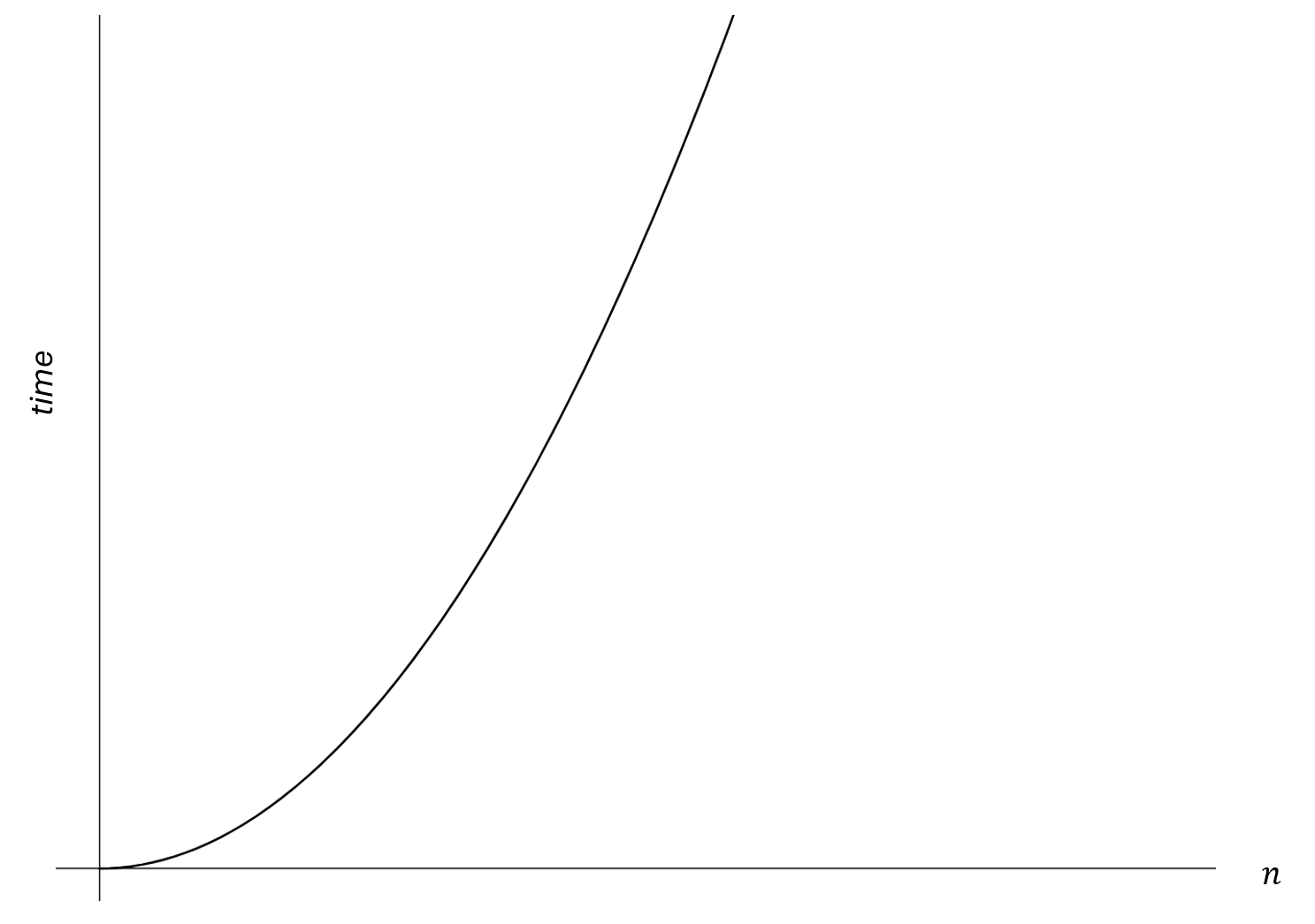
If we were to continue this table and plot them on a graph, where the axis is the input size and the axis is the time (measured in number of comparisons), we would get this :
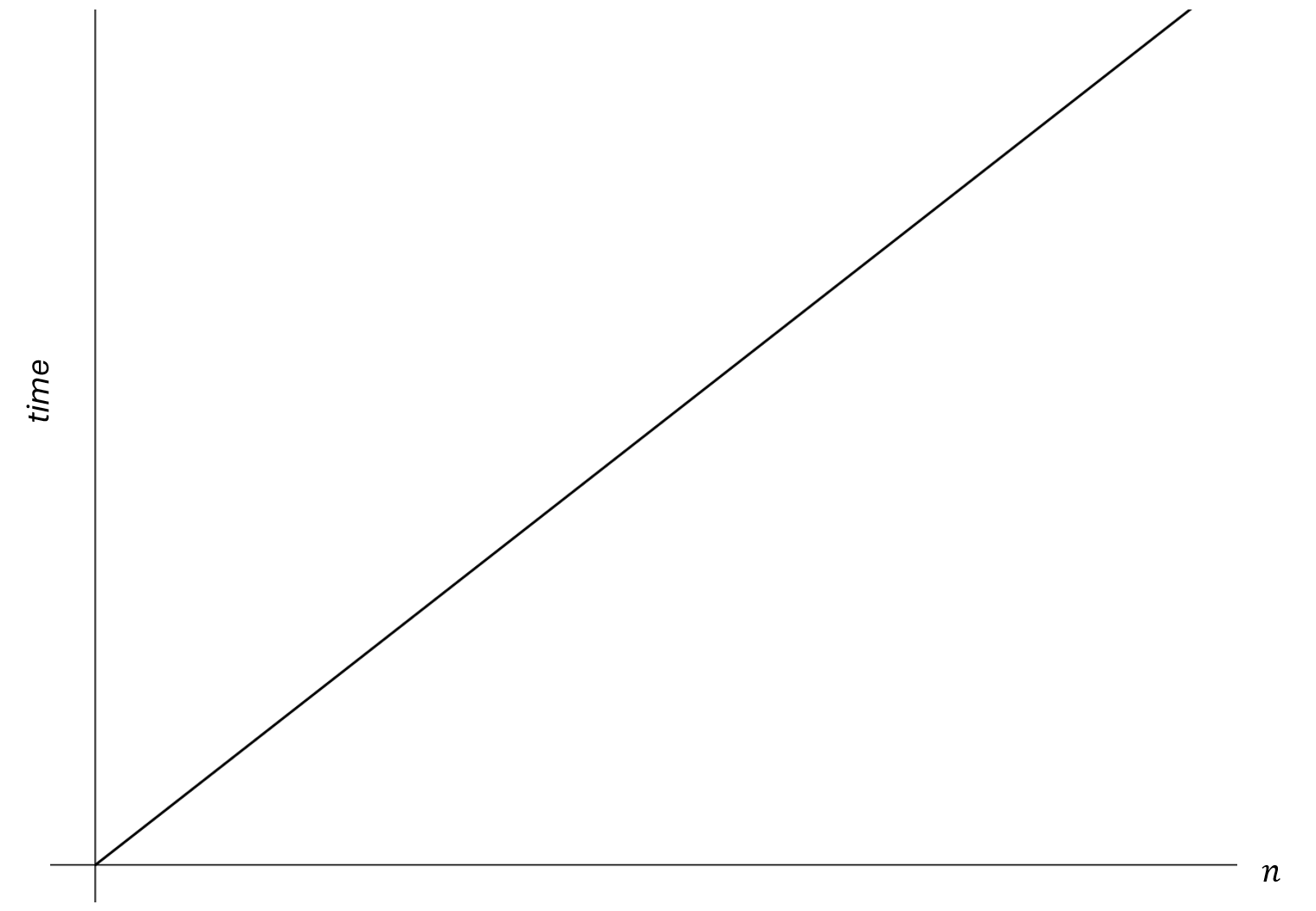
Linear search has linear time complexity, which means that the amount of work is linearly proportional to the input size n.
Big O notation is a mathematical notation used to classify algorithms according to how their running time grows as the input size increases.
Since we concluded that linear search has linear time complexity, it is a algorithm
Constant Time Complexity
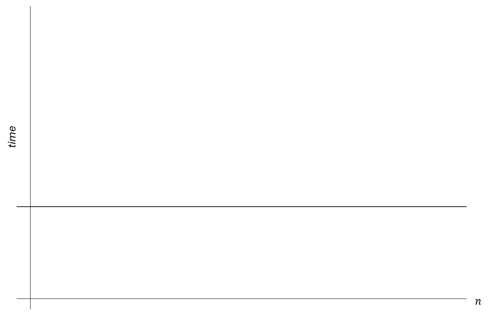
Algorithms said to run in constant time are those whose time complexity does not change regardless of the size of the input. It is denoted as .
For example, imagine an algorithm that returns the first element of a list. Regardless of the size of the list, the first element will always get returned, since there is no additional work required as the input size increases.
Quadratic Time Complexity
Algorithms said to run in quadratic time are those whose time complexity grows quadratically in respect to the input size. It is denoted as .
For example, consider a grid that has rows and columns. The aim of the algorithm is move a token from the starting position of the grid to the end position of the grid. The steps are as follows :
- Start in the bottom row and first column.
- Move the piece to the right by one column but staying on the same row.
- If the piece can't go any further to the right, move it the next row up and start at the first column again.
- Continue these steps until the piece can't go further to the right and cannot go further upwards.
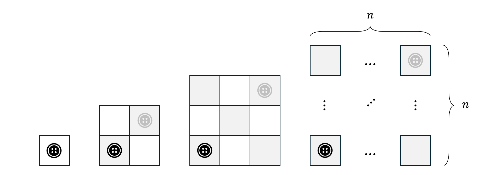
We can see different input sizes for . The work is measured in terms of the number of moves that are needed until the token ends up in the final position (denoted in grey).
| moves | |
|---|---|
| 1 | 1 |
| 2 | 4 |
| 3 | 9 |
From observation we can see that the table follows a quadratic pattern. The time complexity of this algorithm grows quadratically in respect to the input size .
Sorting Algorithms
Sorting is a fundamental operation in computer science with wide-ranging applications across various domains.
It involves arranging data in a specific order, which implies that the nature of the data needs to be comparable.
- Integers are comparable by their magnitude.
- Strings are comparable alphabetically, but can also be compared on their length as well.
- People can be compared on their age, height, weight etc.
There are several sorting algorithms in computer science, the Leaving Certificate syllabus focuses on four specific algorithms for sorting. For each algorithm, you should :
- Outline and identify the steps of the algorithm using different mediums (pseudocode, flowcharts, code etc.)
- Discuss the time complexity of the algorithm.
Selection Sort
Introduction
Selection sort divides the input list into two parts: a sorted part at the left end and an unsorted part at the right end. The algorithm repeatedly selects the smallest (or largest, depending on sorting order) element from the unsorted part and swaps it with the first element of the unsorted part, thereby growing the sorted part by one element and shrinking the unsorted part by one element.
Steps
- Start at the first element of the list.
- Find the smallest element in the unsorted part of the array.
- Swap the found minimum element with the first element of the unsorted part.
- Move the boundary between the sorted and unsorted parts one position to the right and repeat steps 2-3 until the entire array is sorted.
Example
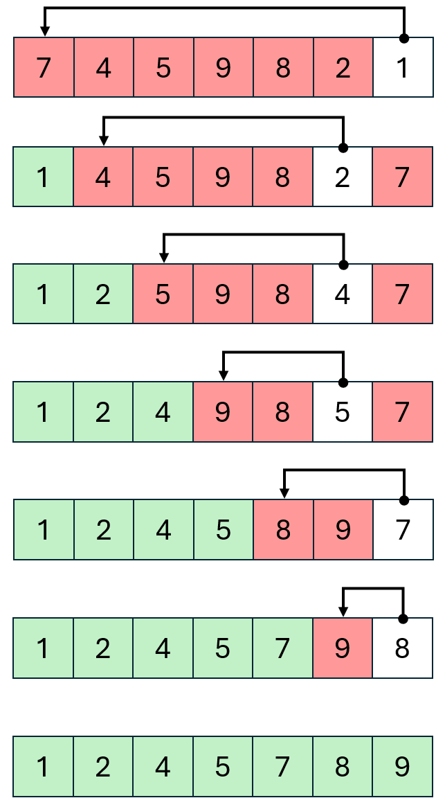
Here is a visual example of selection sort, where red represents the unsorted part of the list, green represents the sorted part of the list and white represents the smallest element found at each iteration.
Implementation
def selection_sort(arr):
    n = len(arr)
    for i in range(n):
        min_index = i
        for j in range(i + 1, n):
            if arr[j] < arr[min_index]:
                min_index = j
        arr[i], arr[min_index] = arr[min_index], arr[i]
    return arr
Time Complexity
Recall that time complexity assumes the worst-case of the algorithm. For a list of size n.
- In the first iteration, the algorithm makes comparisons to find the smallest element.
- In the second iteration, the algorithm makes comparisons to find the smallest element.
- In the last iteration, the algorithm makes comparison to find the smallest element.
The total number of comparisons is which equals to . This can be proved using induction, which is outside of the scope for this chapter.
When deriving time complexity, we ignore constant coefficients and ignore less significant terms.
- We ignore the coefficients of the terms so,
- We ignore terms with lesser powers so,
The time complexity of selection sort is .
Insertion Sort
Introduction
Insertion sort works similarly to the way you might sort playing cards in your hands.
The array is virtually split into a sorted and an unsorted part. Values from the unsorted part are picked and placed at the correct position in the sorted part.
Steps
- Start with the first element (it is trivially sorted).
- Pick the next element.
- Compare the picked element with the elements in the sorted portion.
- Shift all elements in the sorted portion that are greater than the picked element to one position ahead.
- Insert the picked element into the correct position.
- Repeat steps 2 to 5 until all elements are sorted.
Example
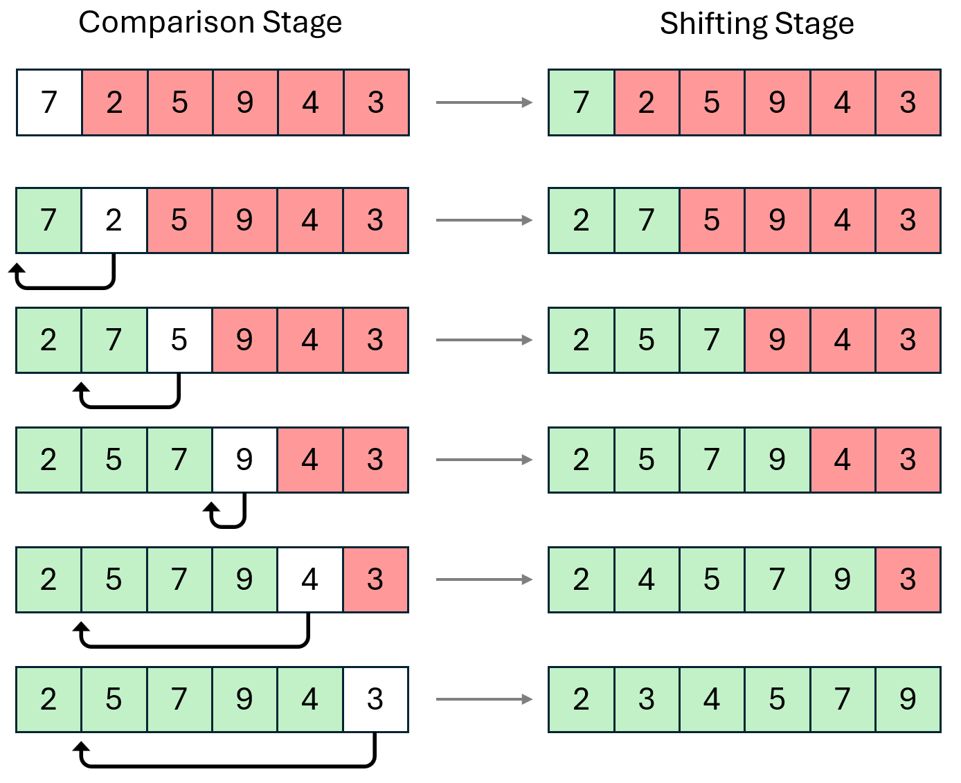
The visual example illustrates two stages for each iteration.
- The comparison stage is where the algorithm finds the position of where to put the element.
- The shifting stage inserts the element into its rightful position, meaning the sub-list to the right of that position needs to be shifted.
Implementation
def insertion_sort(arr):
    # Traverse from arr[1] to arr[n-1]
    for i in range(1, len(arr)):
        key = arr[i]
        j = i - 1
        while j >= 0 and key < arr[j]:
            arr[j + 1] = arr[j]
            j -= 1
        arr[j + 1] = key
    return arr
- Initialisation
- The outer loop iterates over each element in the array starting from the second element (index 1).
- Key Element
- The key element (
key = arr[i]) is the element to be inserted into the sorted portion of the array.
- The key element (
- Inner Loop (Shifting Elements)
- The inner loop (
while j >= 0 and key < arr[j]) shifts elements that are greater than the key one position to the right. - The comparison (
key < arr[j]) ensures that we find the correct position for the key.
- The inner loop (
- Insertion
- After shifting elements, the key is placed in its correct position (
arr[j + 1] = key).
- After shifting elements, the key is placed in its correct position (
Time Complexity
In the worst-case scenario, the array is sorted in reverse order. This means that each element has to be compared with all previous elements, leading to the maximum number of comparisons and shifts.
- First Iteration
- Inner loop comparisons: (compares with the first element)
- Total comparisons so far :
- Second Iteration
- Inner loop comparisons: (compares with the first and second elements)
- Total comparisons so far :
- Third Iteration
- Inner loop comparisons: (compares with the first, second, and third elements)
- Total comparisons so far :
- Iteration:
- Inner loop comparisons: (compares with the first elements)
- Total comparisons so far:
The total number of comparisons made by the inner loop for all iterations of the outer loop is the sum of the first integers.
Again, this can be proved with induction which is outside of the scope for this chapter.
Insertion sort has a time complexity of .
You might have noticed that algorithms involving a nested loop have time complexities of .
Bubble Sort
Introduction
Bubble sort repeatedly steps through the list, compares adjacent elements, and swaps them if they are in the wrong order. The pass through the list is repeated until the list is sorted.
Steps
- Compare adjacent elements : Start with the first element and compare it with the next element.
- Swap elements : If the first element is greater than the next element, swap them.
- Move to the next pair : Continue this process for the next pair of adjacent elements, and so on, until the end of the list.
- Repeat the process : Repeat steps 1 to 3 for all elements in the list until no swaps are needed.
Example
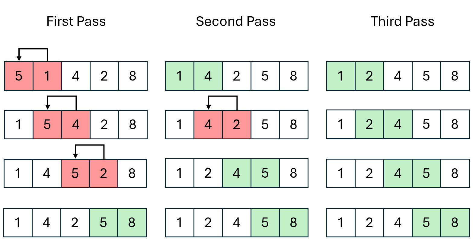
Each pass involves comparing each pair of adjacent elements. Red indicates that these pairs are in the wrong order, which need to be swapped and green indicates that these pairs are in the right order and don't need to be swapped.
Implementation
def bubble_sort(arr):
    n = len(arr)
    for i in range(n):
        # Track whether any swaps were made during this iteration
        swapped = False
        for j in range(0, n-i-1):
            if arr[j] > arr[j+1]:
                arr[j], arr[j+1] = arr[j+1], arr[j]
                swapped = True
        # If no swaps were made, the array is already sorted
        if not swapped:
            break
    return arr
- Initialisation
- The outer loop iterates over each element in the array.
- Swapping Elements
- The inner loop compares adjacent elements and swaps them if they are in the wrong order.
- A flag (
swapped) is used to track whether any swaps were made during the current iteration.
- Optimising
- If no swaps are made during an iteration, the array is already sorted, and the loop can be terminated early.
Time Complexity
- The outer loop runs times.
- The inner loop runs up to times in the worst case for each iteration of the outer loop.
- The total number of comparisons in the worst case is the sum of the first integers, which is .
Bubble sort has a time complexity of .
Quick Sort
Introduction
Quicksort is a divide-and-conquer algorithm that works by selecting a "pivot" element from an array and partitioning the other elements into two sub-arrays, according to whether they are less than or greater than the pivot.
Steps
- Select an element from the array as the pivot. Common strategies include picking the first element, the last element, the middle element, or a random element.
- Rearrange the array so that all elements less than the pivot come before it, and all elements greater than the pivot come after it. The pivot is now in its final sorted position.
- Recursively apply the above steps to the sub-array of elements with smaller values and the sub-array of elements with larger values.
Example
In this example, blue represents the pivot elements.
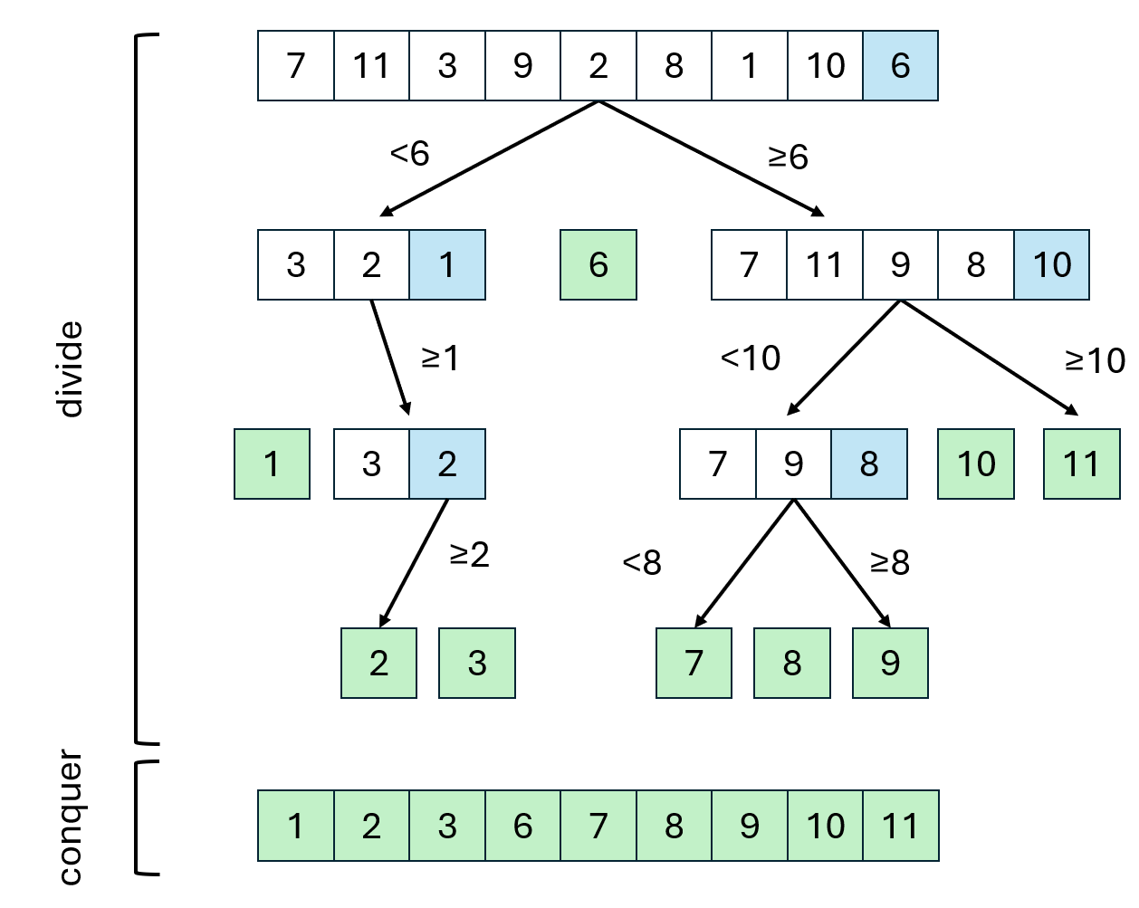
Note that the pivot doesn't necessarily have to be the last element.
Implementation
def quicksort(arr):
    # Base case: if the array is empty or has one element, it's already sorted
    if len(arr) <= 1:
        return arr

    # Choose a pivot element
    pivot = arr[len(arr) - 1]

    # Partition the array into three lists
    left = [x for x in arr if x < pivot]
    middle = [x for x in arr if x == pivot]
    right = [x for x in arr if x > pivot]

    # Recursively sort the left and right sub-arrays and combine the results
    return quicksort(left) + middle + quicksort(right)
- Base Case
- The function checks if the array has one or zero elements and returns it as sorted.
- Pivot Selection
- The pivot is chosen as the last element (
arr[len(arr) - 1]) for simplicity.
- The pivot is chosen as the last element (
- Partitioning
- The array is divided into
left,middle, andrightbased on comparison with the pivot. leftcontains elements less than the pivot.middlecontains elements equal to the pivot.rightcontains elements greater than the pivot.
- The array is divided into
- Recursive Calls
- The function calls itself recursively on the
leftandrightarrays, then combines the sortedleft,middle, andrightarrays to form the final sorted array.
- The function calls itself recursively on the
Time Complexity
- The worst case occurs when the pivot consistently results in unbalanced partitions, such as when the smallest or largest element is always chosen as the pivot.
- This results in a recursion depth of 𝑛 and a quadratic time complexity.
Quick sort has a time complexity of .
Searching Algorithms
The Leaving Certificate focuses on two searching algorithms, linear search and binary search. We have already seen linear search earlier in the chapter including its time complexity.
Binary Search
Introduction
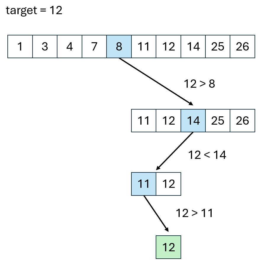
Binary search works by repeatedly dividing the search interval in half, which makes it much faster than linear search for large datasets.
Steps
- Start with two pointers or indices:
leftat the beginning of the array andrightat the end. - Calculate the midpoint index between
leftandright. - If the target value equals the element at the midpoint, the search is complete, and the index is returned.
- If the target value is less than the element at the midpoint, adjust the
rightboundary tomid - 1, narrowing the search to the left half. - If the target value is greater than the element at the midpoint, adjust the
leftboundary tomid + 1, narrowing the search to the right half.
- If the target value is less than the element at the midpoint, adjust the
- Repeat the process until the target is found or the
leftpointer surpasses therightpointer, indicating that the target is not present in the array.
Example
In this example, the blue represents the midpoint element.
Implementation
def binary_search(arr, target):
    left, right = 0, len(arr) - 1

    while left <= right:
        mid = left + (right - left) // 2  # Calculate the mid-point

        # Check if the target is at the mid-point
        if arr[mid] == target:
            return mid  # Target found

        # Adjust the search range
        elif arr[mid] < target:
            left = mid + 1  # Search in the right half
        else:
            right = mid - 1  # Search in the left half

    return -1  # Target not found
- Initialisation
- The function initialises two pointers,
leftandright, to the start and end of the array.
- The function initialises two pointers,
- Iterative Search
- It enters a
whileloop that continues as long asleftis less than or equal toright.
- It enters a
- Midpoint Calculation
- The midpoint is calculated using
left + (right - left) // 2to prevent potential overflow issues.
- The midpoint is calculated using
- Comparison and Adjustment
- If the element at
midequals the target, the indexmidis returned. - If the target is less than the element at
mid, therightboundary is updated tomid - 1. - If the target is greater, the
leftboundary is updated tomid + 1.
- If the element at
- Termination
- If the loop exits without finding the target, the function returns -1, indicating the target is not in the array.