Short Run Costs (Grade 11 NSC Matric Economics): Revision Notes
Short Run Costs
What is the short run?
The short run is a specific time period in production where at least one factor of production cannot be changed. During this period, businesses can only adjust their output by increasing or decreasing the use of variable factors.
Think of it this way: imagine you own a small bakery in Cape Town. In the short run, you cannot change the size of your shop or buy new ovens immediately. These are your fixed factors. However, you can hire more workers, buy more flour, or use more electricity to increase production. These are your variable factors.
Understanding different types of costs
Fixed costs
Fixed costs are expenses that remain constant regardless of how much you produce. These costs don't change whether you make 10 loaves of bread or 100 loaves.
Key characteristics of fixed costs:
- Stay the same at all production levels
- Must be paid even if production is zero
- Include rent, insurance, loan payments, and equipment costs
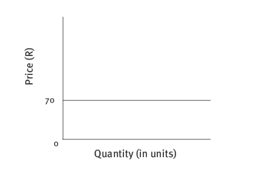
The graph above shows how fixed costs remain constant - they appear as a horizontal line because they don't change with quantity produced.
Formula: Average fixed costs:
Where TFC = Total fixed costs and Q = Output
An important point to remember is that average fixed costs fall as output increases. This happens because you're spreading the same fixed cost over more units of production.
It's like sharing pizza costs among friends - the more friends, the less each person pays!
Variable costs
Variable costs change directly with the level of output. The more you produce, the higher these costs become.
Examples of variable costs:
- Raw materials (flour, sugar for our bakery)
- Labour wages for extra workers
- Electricity for production
- Packaging materials
Formula: Average variable costs:
Where TVC = Total variable costs and Q = Output
Total costs
Total costs represent the complete expense of production, combining both fixed and variable elements.
Formulas:
Where TC = Total cost, FC = Fixed costs, VC = Variable costs, ATC = Average total cost, Q = Output
Worked Example: Fruit Canning Company Cost Analysis
Let's examine data from a fruit canning company:
| Quantity of fruit cans (thousands) | Labour units | Fixed cost (R) | Variable cost (R) | Total cost (R) |
|---|---|---|---|---|
| 0 | 0 | 50,000 | 0 | 50,000 |
| 1 | 5 | 50,000 | 5,000 | 55,000 |
| 2 | 10 | 50,000 | 10,000 | 60,000 |
| 3 | 15 | 50,000 | 15,000 | 65,000 |
| 4 | 20 | 50,000 | 20,000 | 70,000 |
| 5 | 25 | 50,000 | 25,000 | 75,000 |
| 6 | 30 | 50,000 | 30,000 | 80,000 |
Notice how fixed costs stay at R50,000 throughout, while variable costs increase by R5,000 for each additional thousand cans produced.
Marginal costs
Marginal cost is the additional expense incurred when producing one extra unit of output. It tells us how much total cost increases when we decide to make one more product.
Formula:
Where Δ represents "change in"
Understanding marginal cost helps businesses make important decisions about whether it's profitable to increase production.
Cost curves and their relationships
Cost curves provide visual representations of how different costs behave as output changes. These graphs are essential tools for understanding business economics.
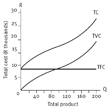
This graph shows three important cost curves:
- TFC (Total Fixed Cost): Remains horizontal because fixed costs don't change
- TVC (Total Variable Cost): Slopes upward as variable costs increase with output
- TC (Total Cost): Slopes upward but starts higher than TVC due to fixed costs
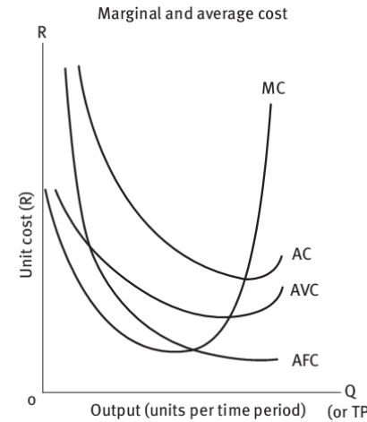
This second graph demonstrates the relationships between average and marginal costs:
- AFC (Average Fixed Cost): Continuously decreases as output increases
- AVC (Average Variable Cost): Typically U-shaped, falling then rising
- AC (Average Cost): U-shaped curve that combines AFC and AVC effects
- MC (Marginal Cost): U-shaped curve that intersects both AC and AVC at their minimum points
Critical relationship: The marginal cost curve always cuts through both the average cost and average variable cost curves at their lowest points. This is a crucial concept for examinations!
The law of diminishing returns
The law of diminishing returns explains why cost curves have their characteristic shapes. It states that when you keep adding more of a variable input (like workers) while keeping other inputs constant (like equipment), eventually each additional unit of the variable input will produce less extra output.
Worked Example: Shoe Factory Production
Here's data from a shoe factory showing diminishing returns:
| Labour units | Total product (pairs) | Marginal product (pairs) |
|---|---|---|
| 1 | 10 | 10 |
| 2 | 22 | 12 |
| 3 | 32 | 10 |
| 4 | 40 | 8 |
| 5 | 44 | 4 |
Analysis:
- Initially, adding workers increases production significantly (marginal product rises from 10 to 12)
- After the second worker, each additional worker contributes less to total output
- By the fifth worker, the marginal product has fallen to just 4 pairs
What's causing this pattern: This happens because there isn't enough equipment for all workers to be fully productive. Some workers might be waiting for machines or getting in each other's way.
Practical applications for businesses
Understanding short run costs helps South African businesses make better decisions:
For pricing decisions:
- Knowing marginal cost helps determine if it's profitable to accept additional orders
- Understanding average costs helps set competitive prices
For production planning:
- Recognising when diminishing returns set in helps optimise workforce size
- Understanding fixed cost behaviour helps with budgeting and planning
For efficiency improvements:
- Monitoring average variable costs can identify areas for operational improvements
- Tracking marginal costs helps determine optimal production levels
Key Points to Remember:
- Fixed costs remain constant regardless of output level, but average fixed costs decrease as production increases
- Variable costs change directly with output, and their behaviour determines the shape of marginal cost curves
- Marginal cost curves intersect average cost curves at their minimum points - this is a key examination concept
- The law of diminishing returns explains why marginal costs eventually rise as more variable inputs are added
- Cost curve analysis is essential for business decision-making, helping determine optimal production levels and pricing strategies