The Individual Business and the Industry (Grade 12 NSC Matric Economics): Revision Notes
The Individual Business and the Industry
Understanding how individual businesses operate within perfectly competitive markets is crucial for grasping microeconomic principles. In perfect competition, individual firms face unique constraints and opportunities that shape their decision-making processes.
Determining the market price
In perfect competition, the market price is determined through the interaction of industry-wide supply and demand forces, not by individual businesses. This creates a two-part analysis that helps us understand how prices are established and how individual firms respond.
Understanding price determination requires analysing both the entire industry (macroeconomic view) and individual firms (microeconomic view) simultaneously. This dual perspective is essential for comprehending how perfect competition works in practice.
Industry vs individual producer analysis
To understand price determination, economists use two side-by-side graphs. The left graph shows the entire industry, where supply and demand curves intersect to determine the market price. The right graph shows how an individual producer responds to this market-determined price.
The industry graph demonstrates market forces in equilibrium. When the demand and supply curves intersect, they establish the market price that all firms must accept. This equilibrium point shows where the quantity demanded equals the quantity supplied across the entire market.
Individual producers cannot influence this market price because they represent only a tiny fraction of total market activity. They become "price takers" - meaning they must accept whatever price the market determines. This is a fundamental characteristic that distinguishes perfect competition from other market structures.
Price-Taking Behavior
Individual firms in perfect competition are price takers because:
- They represent a negligible fraction of total market supply
- They have no market power to influence prices
- They must accept the market-determined price or lose all customers
The price-taking phenomenon
Since individual firms cannot influence the market price, they face a perfectly elastic demand curve. This means they can sell any quantity they choose at the market price, but they cannot charge more or less without losing all customers or profits respectively.
Demand curve for an individual producer
The demand curve facing an individual producer in perfect competition appears as a horizontal straight line at the market price level. This horizontal line represents several important economic concepts simultaneously.
Understanding the revenue relationships
In perfect competition, a remarkable relationship exists where demand equals average revenue equals marginal revenue equals price (D = AR = MR = P). This equality occurs because the firm can sell additional units without affecting the price.
The Fundamental Revenue Relationship
In perfect competition: D = AR = MR = P
This means:
- Demand (D) = horizontal line at market price
- Average Revenue (AR) = = price per unit
- Marginal Revenue (MR) = = revenue from each additional unit
- Price (P) = market-determined price
All four measures are equal and constant!
Let's examine this through numerical examples:
Worked Example: Revenue Relationships in Perfect Competition
| Quantity | Price (P) | Total Revenue | Marginal Revenue (MR = ΔTR/ΔQ) | Average Revenue (AR = TR/Q) |
|---|---|---|---|---|
| 0 | 5 | 0 | 5 | 5 |
| 1 | 5 | 5 | 5 | 5 |
| 2 | 5 | 10 | 5 | 5 |
| 3 | 5 | 15 | 5 | 5 |
| 4 | 5 | 20 | 5 | 5 |
| 5 | 5 | 25 | 5 | 5 |
| 6 | 5 | 30 | 5 | 5 |
Analysis: Each additional unit sold adds exactly R5 to total revenue (marginal revenue), and the average revenue per unit remains R5 regardless of quantity sold.
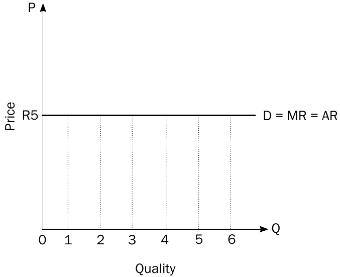
The perfectly elastic demand curve shows that consumers will buy any quantity the firm produces at the market price of R5, but they will buy nothing if the price rises above R5, and the firm has no incentive to charge below R5.
Profit maximisation
Profit maximisation is the primary objective for firms in perfect competition. There are two equivalent methods to determine the profit-maximising output level, both leading to the same optimal production quantity.
The Golden Rule of Profit Maximisation
Profit maximisation occurs where MR = MC
This rule applies because:
- When MR > MC: each additional unit increases profit
- When MR = MC: profit is maximised
- When MR < MC: each additional unit decreases profit
Method 1: marginal revenue equals marginal cost (MR = MC)
The first approach compares marginal revenue with marginal cost. This method recognises that firms should continue producing as long as each additional unit adds more to revenue than it adds to costs.
Worked Example: MR = MC Method
| Quantity | Price | Marginal Revenue | Marginal Cost | Contribution to Profits |
|---|---|---|---|---|
| 1 | 5 | 5 | 2 | 3 |
| 2 | 5 | 5 | 3 | 2 |
| 3 | 5 | 5 | 4 | 1 |
| 4 | 5 | 5 | 5 | 0 |
| 5 | 5 | 5 | 6 | -1 |
| 6 | 5 | 5 | 7 | -2 |
Solution: Profit maximisation occurs at 4 units of output, where MR = MC = 5. Beyond this point, marginal cost exceeds marginal revenue, reducing overall profits.
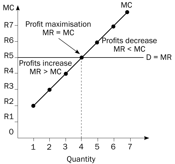
The graphical representation clearly shows three distinct regions:
- Left of equilibrium (MR > MC): Profits increase with additional production
- At equilibrium (MR = MC): Profit maximisation achieved
- Right of equilibrium (MR < MC): Profits decrease with additional production
Method 2: total revenue minus total cost (TR - TC)
The second approach examines the difference between total revenue and total cost, seeking the output level where this difference is greatest.
Alternative Approach: TR - TC Method
This method finds the same profit-maximising output by identifying where the gap between total revenue and total cost is largest. While the MR = MC method shows the marginal decision-making process, the TR - TC method shows the overall profit picture.
Worked Example: TR - TC Method
| Quantity | Price | Total Revenue | Total Cost | Profit (TR - TC) |
|---|---|---|---|---|
| 0 | 5 | 0 | 1 | -1 |
| 1 | 5 | 5 | 3 | 2 |
| 2 | 5 | 10 | 6 | 4 |
| 3 | 5 | 15 | 10 | 5 |
| 4 | 5 | 20 | 15 | 5 |
| 5 | 5 | 25 | 21 | 4 |
| 6 | 5 | 30 | 28 | 2 |
Analysis: Maximum profit of R5 occurs at both 3 and 4 units. Economic theory identifies 4 units as the precise profit-maximising output because this is where MR = MC.
Interpreting profit maximisation results
Both methods demonstrate important business principles. When total cost exceeds total revenue, the business operates at a loss. Maximum profit is achieved when the gap between total revenue and total cost is largest. Once maximum profit is reached, additional production reduces overall profitability.
The graphical analysis shows total cost and total revenue curves, with profit represented by the vertical distance between them. The widest gap between these curves indicates the profit-maximising output level.
Why Firms Don't Always Produce More
Even though a firm could potentially sell more units in perfect competition, producing beyond the profit-maximising point would increase total revenue but increase total costs by even more, resulting in lower overall profits. This explains why profit-maximising firms voluntarily limit their production.
Practical applications
Understanding profit maximisation helps businesses make informed production decisions. In perfectly competitive markets, firms must carefully balance their production costs against the fixed market price to optimise their profitability.
This analysis explains why businesses might limit their production even when they could sell more units. Producing beyond the profit-maximising point would increase total revenue but would increase total costs by even more, resulting in lower overall profits.
Key Points to Remember:
-
Individual firms in perfect competition are price takers - they must accept the market-determined price and cannot influence it
-
The demand curve facing individual firms is perfectly elastic - horizontal line showing D = AR = MR = P
-
Profit maximisation occurs where MR = MC - this is the fundamental rule for optimal production decisions
-
Two equivalent methods exist for finding profit-maximising output - comparing MR with MC, or finding where TR - TC is maximum
-
Producing beyond the profit-maximising point reduces total profits - even though total revenue continues to increase, costs increase faster