Curve Fitting (Grade 12 NSC Matric Mathematics): Revision Notes
Curve Fitting
Introduction to curve fitting
Curve fitting is the process of identifying the mathematical relationship between two variables by examining their scatter plot pattern. When we have bivariate data (data involving two variables), we can plot these as points on a coordinate system to create a scatter plot.
Scatter plots allow us to visualise the direction and strength of relationships between variables:
Understanding relationship characteristics is fundamental to curve fitting:
- Direction: A relationship is positive if high values of one variable occur with high values of the other, or negative if high values of one variable occur with low values of the other
- Strength: A relationship is strong if data points lie close to a recognisable pattern, or weak if points are scattered further from the pattern
Types of relationships
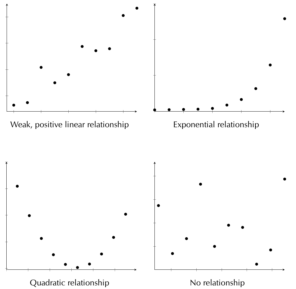
When examining scatter plots, we can identify several common relationship patterns that help determine the most appropriate mathematical model for our data:
Linear relationships
- Strong positive linear: Points form a clear upward trend from left to right
- Strong negative linear: Points form a clear downward trend from left to right
- Weak positive linear: Points show an upward trend but with more scatter
- Weak negative linear: Points show a downward trend but with more scatter
Non-linear relationships
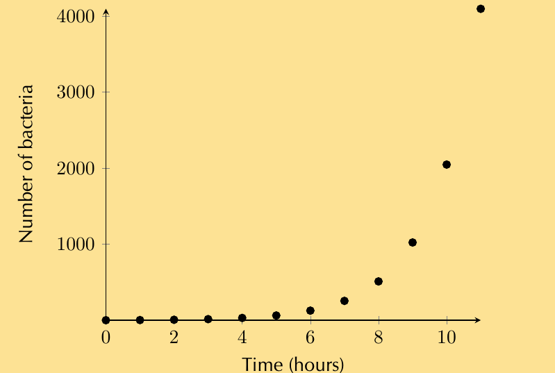
- Exponential: Points form a curved pattern that increases rapidly (or decreases rapidly for negative exponential)
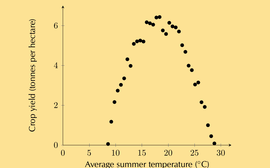
- Quadratic: Points form a U-shaped or inverted U-shaped curve (parabola)
No relationship
- Points appear randomly scattered with no recognisable pattern
Pattern Recognition Tip: Look for the overall trend first - does it go up, down, or curve? Then assess how closely the points follow that trend to determine strength.
Intuitive curve fitting
For simple datasets, we can draw a line of best fit (also called a trend line) by hand. This line should pass as close as possible to all data points, with approximately equal numbers of points above and below the line.
Steps for drawing a line of best fit by hand:
- Plot all data points on a coordinate system
- Draw a straight line that best represents the overall trend
- Ensure the line has roughly equal numbers of points above and below it
- Calculate the equation of the line using two points on the line
The equation of a straight line is:
Where:
- m is the gradient (slope)
- c is the y-intercept
To find the gradient:
Worked Example: Fitting by Hand
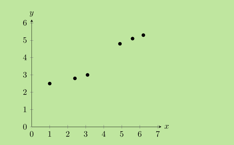
Given the data set with x-values (1.0, 2.1, 3.1, 4.9, 5.6, 6.2) and y-values (2.5, 2.8, 3.0, 4.8, 5.1, 5.3):
Step 1: Plot the data points
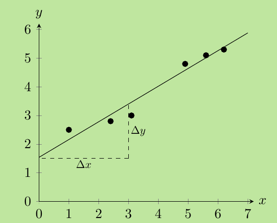
Step 2: Draw a line of best fit through the points
Step 3: Calculate the equation using two points on the line
- If the line passes through (0, 1.5) and (3, 3.5)
- Gradient:
- Equation:
Step 4: Make predictions
- For x = 4 (interpolation):
- For y = 6 (extrapolation): , so
Interpolation and extrapolation
Once we have established a relationship between variables, we can make predictions using two distinct approaches:
Interpolation is predicting values that fall within the range of our existing data. This is generally reliable because we're making predictions based on observed patterns.
Extrapolation is predicting values beyond the range of our data. This must be done with caution unless we're confident the relationship continues beyond our data range.
Critical Distinction:
- Inside the data range = Interpolation (more reliable)
- Outside the data range = Extrapolation (requires caution)
Interpolation is generally trustworthy because you're predicting within observed patterns, while extrapolation assumes the pattern continues beyond your data, which may not always be true.
Linear regression
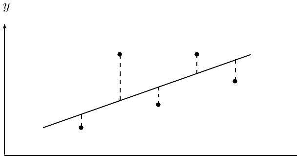
For more precise curve fitting, we use the least squares method. This mathematical technique finds the line that minimises the sum of squared distances between data points and the line.
The least squares regression line has the equation:
Where the coefficients are calculated using:
Where:
- n = number of data points
- = mean of y-values
- = mean of x-values
Worked Example: Least Squares by Hand
For appliance data showing age vs maintenance cost:
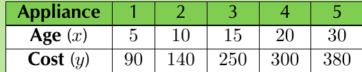
Step 1: Create a calculation table with columns for x, y, xy, and x²
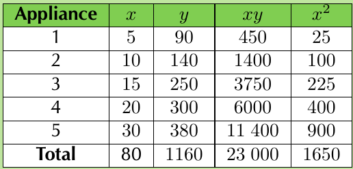
Step 2: Calculate the totals and apply the formulas
- Therefore:
Calculator methods
Scientific calculators can perform linear regression automatically, saving time and reducing calculation errors:
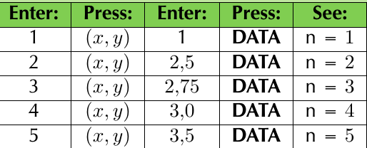
Using SHARP calculator:
- Change mode to "Stat xy"
- Enter data pairs using (x,y) and DATA buttons
- Press RCL then 'a' for y-intercept, RCL then 'b' for gradient
Using CASIO calculator:
- Press MODE and select STAT
- Enter data in X and Y columns
- Access regression menu to get coefficients
Calculator Advantage: Different calculator brands have slightly different button sequences, but all modern scientific calculators can perform regression analysis much faster than hand calculations, especially for large datasets.
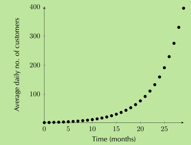
Real-world applications
Curve fitting has many practical applications across diverse fields, making it a valuable tool for understanding relationships in real-world scenarios:
- Business growth: Modelling customer acquisition over time (often exponential)
- Medical research: Analysing drug effectiveness vs dosage
- Agriculture: Understanding optimal growing conditions
- Economics: Studying relationships between variables like price and demand
Common Exam Traps and Tips:
- Always check whether you're interpolating or extrapolating - this affects the reliability of predictions
- Look at the scatter pattern carefully before choosing a function type
- Round final answers appropriately - usually to 2 decimal places unless specified otherwise
- Remember that correlation doesn't imply causation - just because two variables are related doesn't mean one causes the other
- When extrapolating, state any assumptions you're making about the continued pattern
Key Points to Remember:
- Curve fitting identifies mathematical relationships between two variables using scatter plots
- Strong relationships have points close to a recognisable pattern; weak relationships have more scattered points
- Interpolation (predicting within data range) is more reliable than extrapolation (predicting beyond data range)
- The least squares method gives the most accurate line of best fit by minimising squared distances
- Different relationship types require different mathematical models: linear (), exponential, or quadratic
- Calculator methods provide quick and accurate regression analysis for complex datasets