Revision Revision Notes for Grade 12 NSC Matric Mathematics

Revision

Statistical terminology

Statistics helps us understand and describe data sets through various measures. These measures fall into two main categories: measures of central tendency and measures of dispersion.

Measures of central tendency

Measures of central tendency show us where the centre or middle of our data lies. They help us understand the typical or average value in a data set.

The mean represents the arithmetic average of all data values. To calculate the mean, we add all values together and divide by the number of entries:

Mean formula: $\bar{x} = \frac{\sum x_i}{n}$

where $x_i$ represents each data value and $n$ represents the total number of data entries. We read $\bar{x}$ as "x bar".

infoNote

The mean is sensitive to extreme values (outliers) because it includes every data point in its calculation. A single very high or very low value can significantly shift the mean away from the typical data values.

The median is the middle value when data is arranged in ascending or descending order. To find the median, first sort your data from smallest to largest, then locate the middle position. If you have an even number of values, the median equals the average of the two middle values.

Measures of dispersion

Measures of dispersion tell us how spread out our data values are. When dispersion is small, data points cluster closely together. When dispersion is large, data points are scattered across a wider range.

The range represents the simplest measure of spread. It equals the difference between the maximum and minimum values in the data set.

Range = Maximum value - Minimum value

The inter-quartile range measures the spread of the middle 50% of data. Quartiles divide ordered data into four equal parts. The first quartile ( $Q_1$ ) marks the 25% position, the second quartile ( $Q_2$ ) is the median at 50%, and the third quartile ( $Q_3$ ) marks the 75% position.

To find quartile positions when data is numbered from 1, use these formulas:

Location of $Q_1$ = $\frac{1}{4}(n-1) + 1$
Location of $Q_2$ = $\frac{1}{2}(n-1) + 1$
Location of $Q_3$ = $\frac{3}{4}(n-1) + 1$

Inter-quartile range = $Q_3 - Q_1$

chatImportant

The inter-quartile range is less affected by outliers than the range because it focuses on the middle 50% of data and ignores extreme values at both ends.

The variance measures the average squared distance between each data point and the mean. This gives us a precise measure of how much data values deviate from the centre.

Variance formula: $\sigma^2 = \frac{\sum (x_i - \bar{x})^2}{n}$

The standard deviation is simply the square root of variance. It measures spread in the same units as the original data, making it easier to interpret.

Standard deviation formula: $\sigma = \sqrt{\frac{\sum (x_i - \bar{x})^2}{n}}$

Five number summary and box plots

The five number summary combines central tendency and dispersion measures into a comprehensive data description. It includes five key values in this specific order:

Minimum - smallest data value
First quartile ( $Q_1$ ) - 25th percentile
Median ( $Q_2$ ) - 50th percentile
Third quartile ( $Q_3$ ) - 75th percentile
Maximum - largest data value

A box and whisker plot (or box plot) provides a visual representation of the five number summary.

infoNote

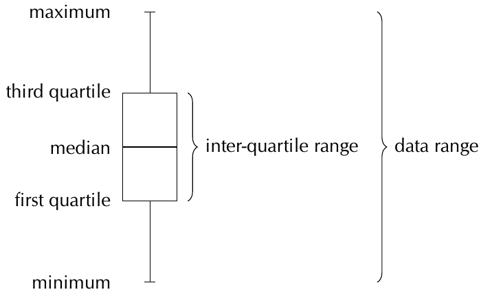
Understanding Box Plot Components:

The rectangular box spans from $Q_1$ to $Q_3$ , showing where the middle 50% of data lies. The line inside the box marks the median position. The whiskers extend from the box to the minimum and maximum values, showing the full data range.

Worked example: Five number summary

lightbulbExample

Worked Example: Constructing a Box Plot

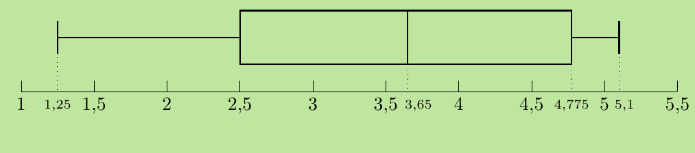
Let's work through constructing a box plot using this data set: 1.25; 1.5; 2.5; 2.5; 3.1; 3.2; 4.1; 4.25; 4.75; 4.8; 4.95; 5.1

Step 1: Find minimum and maximum Since the data is already ordered: Minimum = 1.25, Maximum = 5.1

Step 2: Calculate quartile positions With $n = 12$ values:

Location of $Q_2 = \frac{1}{2}(12-1) + 1 = \frac{1}{2}(11) + 1 = 6.5$

The median lies between the 6th and 7th values (3.2 and 4.1): $Q_2 = \frac{3.2 + 4.1}{2} = 3.65$

Location of $Q_1 = \frac{1}{4}(12-1) + 1 = \frac{1}{4}(11) + 1 = 3.75$

$Q_1$ lies between the 3rd and 4th values (2.5 and 2.5): $Q_1 = \frac{2.5 + 2.5}{2} = 2.5$

Location of $Q_3 = \frac{3}{4}(12-1) + 1 = \frac{3}{4}(11) + 1 = 9.25$

$Q_3$ lies between the 9th and 10th values (4.75 and 4.8): $Q_3 = \frac{4.75 + 4.8}{2} = 4.775$

Step 3: Construct the box plot Five number summary: (1.25; 2.5; 3.65; 4.775; 5.1)

Worked example: Variance and standard deviation calculation

lightbulbExample

Worked Example: Calculating Variance and Standard Deviation

Consider this data set representing coin flip results: {44; 49; 52; 62; 53; 48; 54; 49; 46; 51}

Step 1: Calculate the mean $\bar{x} = \frac{44 + 49 + 52 + 62 + 53 + 48 + 54 + 49 + 46 + 51}{10} = \frac{508}{10} = 50.8$

Step 2: Calculate variance using a table

Table

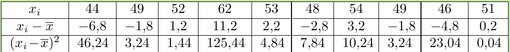
We subtract the mean from each data value, then square the result. The variance equals the sum of squared deviations divided by $n$ :

$\sigma^2 = \frac{225.6}{10} = 22.56$

Step 3: Calculate standard deviation $\sigma = \sqrt{22.56} = ±4.75$

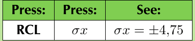
Using a calculator for statistical calculations

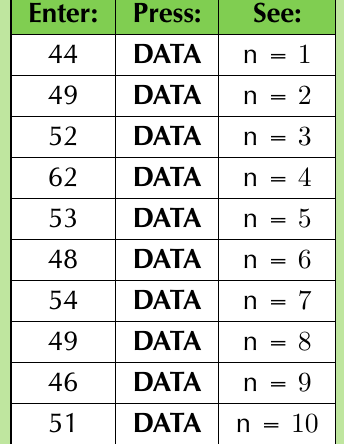
Most scientific calculators can compute these statistics automatically. The general process involves:

Switch to statistical mode
Enter each data value followed by the DATA button
Use statistical functions to recall mean, standard deviation, and other measures

infoNote

While calculators can speed up calculations, understanding the manual process helps you verify results and understand what the statistics actually represent.

Distribution characteristics

Understanding the shape of data distributions helps us interpret statistical results and make predictions about populations.

Symmetric distributions

A symmetric distribution has balanced left and right sides around the mean. The histogram appears roughly bell-shaped with equal tails on both sides.

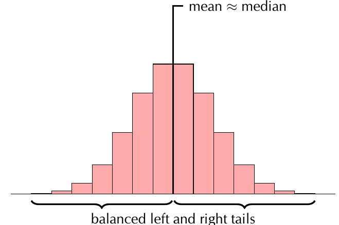
In symmetric distributions, the mean approximately equals the median because the data is evenly balanced around the centre point.

Normal distributions

When large amounts of data are collected from a population, distributions often form a normal distribution (bell curve). This special type of symmetric distribution follows the empirical rule:

chatImportant

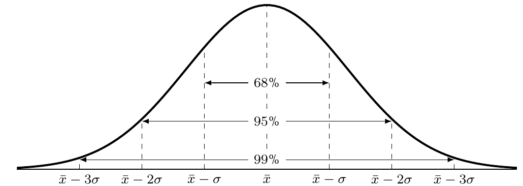
Empirical rule (68-95-99.7 rule):

68% of data falls within 1 standard deviation of the mean ( $\bar{x} ± \sigma$ )
95% of data falls within 2 standard deviations of the mean ( $\bar{x} ± 2\sigma$ )
99.7% of data falls within 3 standard deviations of the mean ( $\bar{x} ± 3\sigma$ )

This rule helps us understand how spread out data is and identify unusual values (outliers).

Skewed distributions

Real data doesn't always form symmetric patterns. When distributions have unequal tails, we call them skewed.

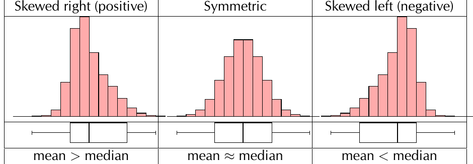
Positively skewed (skewed right):

The mean is greater than the median
The tail extends further to the right
The median is closer to $Q_1$ than to $Q_3$
Common when there are a few very high scores

Negatively skewed (skewed left):

The mean is less than the median
The tail extends further to the left
The median is closer to $Q_3$ than to $Q_1$
Common when there are a few very low scores

infoNote

Memory Aid for Skewness: Think of the direction the tail points - if the tail points right, it's positively skewed (skewed right). If the tail points left, it's negatively skewed (skewed left).

Worked example: Comparing distributions

lightbulbExample

Worked Example: Analysing Three Class Distributions

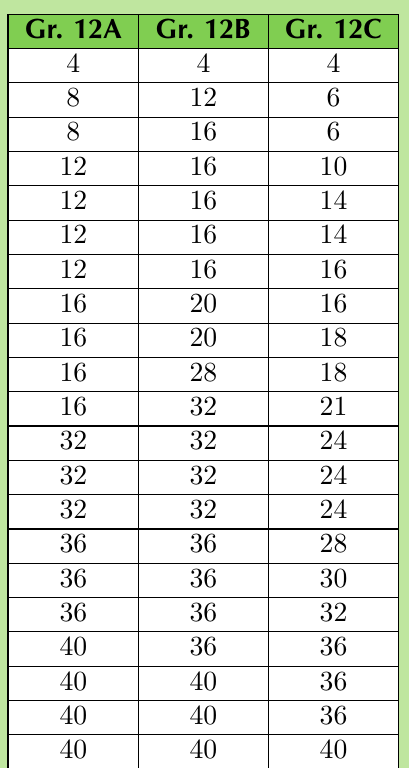
Three Grade 12 classes wrote a mathematics test out of 40 marks. Let's analyse their performance:

Table

Solution:

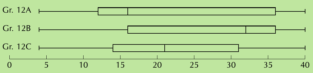
First, we calculate the five number summary for each class:

Gr. 12A: [4; 12; 16; 36; 40]
Gr. 12B: [4; 16; 32; 36; 40]
Gr. 12C: [4; 14; 21; 31; 40]

Statistical calculations:

Gr. 12A: Mean = 23.6, Standard deviation = ±12.70
Gr. 12B: Mean = 26.5, Standard deviation = ±10.65
Gr. 12C: Mean = 21.6, Standard deviation = ±10.54

Distribution analysis:

Gr. 12A: Mean (23.6) > Median (16) → Positively skewed The class had many low marks with some high achievers pulling the mean upward.

Gr. 12B: Mean (26.5) < Median (32) → Negatively skewed
The class performed well overall with a few low marks pulling the mean downward.

Gr. 12C: Mean (21.6) ≈ Median (21) → Approximately symmetric The class had a balanced distribution of high and low marks.

bookmarkSummary

Key Points to Remember:

Mean = sum of all values ÷ number of values; affected by extreme values
Median = middle value when data is ordered; less affected by outliers
Standard deviation measures spread around the mean; larger values indicate more variability
Box plots visually display the five number summary and help identify distribution shape
Skewness direction: If mean > median, distribution is positively skewed (right tail longer); if mean < median, distribution is negatively skewed (left tail longer)
The 68-95-99.7 rule applies to normal distributions and helps identify outliers

Revision (Grade 12 NSC Matric Mathematics): Revision Notes

Revision

Statistical terminology

Measures of central tendency

Measures of dispersion

Five number summary and box plots

Worked example: Five number summary

Worked example: Variance and standard deviation calculation

Using a calculator for statistical calculations

Distribution characteristics

Symmetric distributions

Normal distributions

Skewed distributions

Worked example: Comparing distributions

Explore Grade 12 NSC Matric Mathematics Model Answers by Topics

Trigonometry

Analytical Geometry

Euclidean Geometry

Statistics

Probability

Explore Grade 12 NSC Matric Mathematics Quizzes by Topics

Trigonometry

Analytical Geometry

Euclidean Geometry

Statistics

Probability

Explore Grade 12 NSC Matric Mathematics Flashcards by Topics

Trigonometry

Analytical Geometry

Euclidean Geometry

Statistics

Probability

Join 100,000+ NSC Matric students studying Revision Notes with us.