Income-Expenditure Diagram Revision Notes for HSC SSCE Economics

Income-Expenditure Diagram

Introduction

The income-expenditure diagram is a powerful tool for analysing how economies reach equilibrium and how changes in aggregate demand affect national income. It builds on concepts of equilibrium, aggregate demand and supply components, and the multiplier process.

infoNote

This diagram allows economists to visualise the relationship between total spending in an economy and the level of national income, making it easier to understand why economies might experience unemployment or inflation and what governments can do about it.

Structure of the diagram

The income-expenditure diagram (also called the Keynesian cross diagram) has two axes:

Horizontal axis (x-axis): Income $(Y)$
Vertical axis (y-axis): Expenditure $(E)$

The diagram contains two key lines that together determine the economy's equilibrium position.

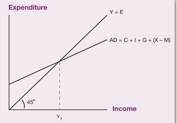
The equilibrium line (Y=E)

The equilibrium line represents all points where expenditure equals income. This is shown as a 45-degree diagonal line from the origin.

Economic significance: When the economy operates on any point along this line, aggregate demand equals aggregate supply. At this point, injections into the economy equal leakages from it, meaning there is no tendency for the economy to change. The economy is in equilibrium.

infoNote

The 45-degree angle occurs because every unit increase in income along the horizontal axis corresponds to an equal unit increase in expenditure on the vertical axis when the two are equal. This geometric property makes it easy to identify where income and expenditure are balanced.

The aggregate demand line

Components of aggregate demand

Aggregate demand represents total planned spending in the economy. It comprises four components:

$\text{AD} = C + I + G + (X - M)$

Where:

$C$ = Consumption expenditure by households
$I$ = Investment expenditure by firms
$G$ = Government spending
$X$ = Exports
$M$ = Imports (subtracted because they represent spending on foreign goods)

How income affects aggregate demand

The relationship between income and aggregate demand is crucial for understanding the diagram. In a simplified model:

Investment $(I)$ , government spending $(G)$ , and net exports $(X-M)$ are considered independent of income levels. These components do not automatically rise or fall when national income changes.
Consumption $(C)$ is the component through which income and expenditure are connected. When households earn more income, they spend more on consumption goods and services.

The consumption function

Consumption can be broken down into two parts:

Autonomous consumption $(C_0)$ : The minimum level of spending that occurs even when income is very low or zero. Households meet their basic needs by drawing on savings or borrowing money.
Induced consumption: The additional consumption that results from earning income. This is calculated as the marginal propensity to consume (MPC) multiplied by income $(Y)$ .

The consumption function is:

$C = C_0 + \text{mpc} \times Y$

Where MPC represents the proportion of each additional dollar of income that households spend on consumption (the rest is saved).

The full aggregate demand equation

Combining the consumption function with the other components gives:

$\text{AD} = C_0 + \text{mpc} \times Y + I + G + (X - M)$

This equation shows that aggregate demand depends partly on autonomous spending $(C_0 + I + G + (X-M))$ and partly on income through the consumption term $(\text{mpc} \times Y)$ .

Characteristics of the aggregate demand line

chatImportant

The AD line has three important features that are essential for understanding how the economy reaches equilibrium:

Upward sloping: As income rises, consumption increases, so total expenditure in the economy rises. The positive relationship between income and expenditure creates an upward slope.
Flatter than 45 degrees: The AD line slopes upward but less steeply than the equilibrium line. This occurs because not all additional income is spent—some leaks into savings. Since MPC is less than 1 (households save a portion of extra income), the AD line is flatter than the 45-degree equilibrium line.
Cuts the y-axis above the origin: Even when income is zero, there is still some expenditure in the economy. This is because autonomous consumption $(C_0)$ , investment $(I)$ , government spending $(G)$ , and net exports $(X-M)$ all occur regardless of income level.

Finding equilibrium

The economy reaches equilibrium at the point where the aggregate demand line intersects the 45-degree equilibrium line. At this intersection point, expenditure equals income, and the economy has no tendency to change. In the diagram, this is shown as $Y_1$ .

Shifts in the aggregate demand line

The position and slope of the AD line can change due to various economic factors.

Factors causing upward shifts

The AD line shifts upward (parallel shift) when there is an increase in any autonomous component of spending:

Rise in consumption (e.g., increased consumer confidence)
Rise in investment (e.g., improved business confidence, lower interest rates)
Rise in government spending (expansionary fiscal policy)
Rise in exports (e.g., stronger foreign demand)
Fall in imports (e.g., consumers buy more domestic goods)

An upward shift in AD leads to a new, higher equilibrium level of national income.

Factors causing downward shifts

The AD line shifts downward when there is a decrease in autonomous spending:

Fall in consumption (e.g., reduced consumer confidence)
Fall in investment (e.g., pessimistic business outlook, higher interest rates)
Fall in government spending (contractionary fiscal policy)
Fall in exports (e.g., weaker foreign demand)
Rise in imports (e.g., consumers buy more foreign goods)

A downward shift in AD leads to a new, lower equilibrium level of national income.

Changes in the slope

The steepness of the AD line depends on the marginal propensity to consume:

Rise in MPC: Makes the AD line steeper. When households spend a larger proportion of additional income, expenditure responds more strongly to income changes.
Fall in MPC: Makes the AD line flatter. When households save a larger proportion of additional income, expenditure responds less strongly to income changes.

Changes in slope affect the size of the multiplier effect.

The multiplier effect

One of the most important insights from the income-expenditure diagram is that changes in aggregate demand lead to magnified changes in national income. This is the multiplier effect.

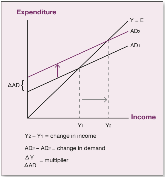
How the multiplier works

When aggregate demand increases (for example, from $\text{AD}_1$ to $\text{AD}_2$ due to higher investment), the economy moves to a new equilibrium. The key observation is that the change in income $(Y_2 - Y_1)$ is larger than the initial change in aggregate demand $(\text{AD}_2 - \text{AD}_1)$ .

infoNote

This multiplication occurs because the initial spending increase triggers a chain reaction:

Higher investment spending increases incomes for those who receive the money
These recipients spend part of their extra income (determined by MPC)
This creates more income for others, who also spend part of it
The process continues, with each round of spending being smaller than the last

The economy eventually settles at a new equilibrium where income has risen by a multiple of the original spending increase.

Calculating the multiplier

The size of the multiplier can be calculated as:

$\text{Multiplier} = \frac{\Delta Y}{\Delta \text{AD}} = \frac{Y_2 - Y_1}{\text{AD}_2 - \text{AD}_1}$

Where:

$\Delta Y$ = change in national income
$\Delta \text{AD}$ = initial change in aggregate demand

The multiplier is larger when the MPC is higher, because more of each extra dollar of income is re-spent in the economy rather than saved.

Output gaps and government intervention

The problem of unemployment equilibrium

chatImportant

The income-expenditure diagram reveals an important insight from economist John Maynard Keynes: an economy can reach equilibrium (where there is no tendency to change) while still experiencing high unemployment.

Equilibrium simply means that aggregate demand equals aggregate supply—it does not guarantee that the economy is operating at full employment. The equilibrium level of income $(Y_e)$ may differ from the full employment level of income $(Y_f)$ .

This creates a role for government policy intervention to shift aggregate demand and move the economy toward full employment.

Deflationary gap

A deflationary gap exists when the equilibrium level of income is below the full employment level $(Y_e < Y_f)$ .

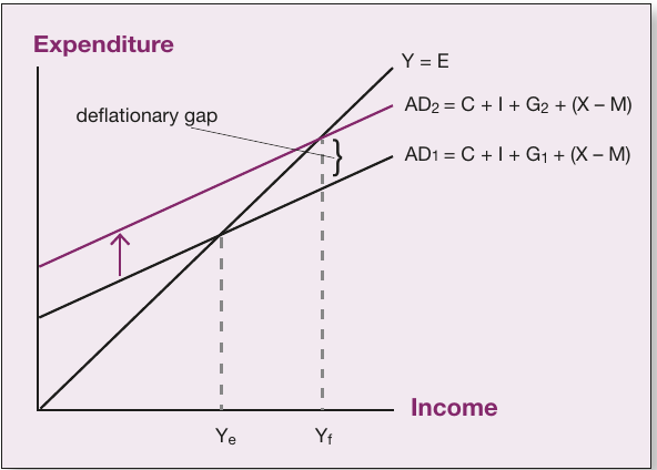
In the diagram above:

$Y_e$ represents the current equilibrium (where $\text{AD}_1$ intersects $Y=E$ )
$Y_f$ represents the full employment level of income
The vertical distance between $\text{AD}_1$ and the 45-degree line at $Y_f$ is the deflationary gap

Economic problem: The economy is producing below its potential, and unemployment is higher than necessary.

infoNote

Policy solution: The government can increase aggregate demand through expansionary policy. In the diagram, increasing government spending from $G_1$ to $G_2$ shifts the AD line upward from $\text{AD}_1$ to $\text{AD}_2$ . Due to the multiplier effect, this boost in government spending increases national income from $Y_e$ to $Y_f$ , achieving full employment.

Inflationary gap

An inflationary gap exists when the equilibrium level of income is above the full employment level $(Y_e > Y_f)$ .

In this scenario:

The economy is operating beyond its sustainable capacity
Unemployment is below the natural rate
Upward pressure on wages and prices creates inflation

infoNote

Policy solution: The government can decrease aggregate demand through contractionary policy. Reducing government spending shifts the AD line downward, bringing income back to the full employment level and containing inflationary pressures.

Why macroeconomic policy matters

At first glance, it might seem that government intervention is unnecessary—after all, the multiplier process automatically adjusts the economy to a new equilibrium after any shock. However, the key issue is that automatic market adjustment does not guarantee the equilibrium will occur at full employment.

Macroeconomic policies (fiscal and monetary policy) are essential tools for:

Reducing unemployment when output is below potential
Controlling inflation when output is above potential
Achieving the government's objectives for economic stability and growth

The income-expenditure diagram provides a clear framework for understanding how these policies work and why they are needed.

Remember!

bookmarkSummary

Key Points to Remember:

The income-expenditure diagram shows the relationship between national income (x-axis) and expenditure (y-axis), with equilibrium occurring where the aggregate demand line intersects the 45-degree $Y=E$ line.
Aggregate demand $(AD = C + I + G + (X-M))$ depends on income through consumption, which equals autonomous consumption plus induced consumption: $C = C_0 + \text{mpc} \times Y$ .
The AD line slopes upward (higher income → higher expenditure) but is flatter than 45° (due to savings leakage) and cuts the y-axis above the origin (due to autonomous spending).
Changes in spending components $(C, I, G, X, M)$ cause parallel shifts in the AD line, while changes in the marginal propensity to consume alter its slope.
The multiplier effect means that initial changes in aggregate demand lead to larger changes in national income, because the initial spending creates a chain reaction of additional spending and income.
A deflationary gap occurs when equilibrium income is below full employment, requiring expansionary policy to increase aggregate demand and reduce unemployment.
An inflationary gap occurs when equilibrium income is above full employment, requiring contractionary policy to decrease aggregate demand and control inflation.

Income-Expenditure Diagram (HSC SSCE Economics): Revision Notes