Price Elasticity of Supply (HSC SSCE Economics): Revision Notes

Price Elasticity of Supply

What is price elasticity of supply?

Price elasticity of supply (PES) indicates how much the quantity supplied of a product changes in response to a change in its price. It measures the sensitivity or responsiveness of producers to price movements.

The price elasticity of supply is calculated as the percentage change in quantity supplied divided by the percentage change in price.

$\text{PES} = \frac{\% \text{ change in quantity supplied}}{\% \text{ change in price}}$

For most goods, when price rises, quantity supplied expands. This means PES is typically positive. However, the size of that response varies considerably between products.

Types of price elasticity of supply

Relatively elastic supply

When quantity supplied changes by a larger percentage than the price change, supply is described as relatively elastic. Producers can respond strongly to price signals by significantly increasing or decreasing output.

Relatively inelastic supply

When quantity supplied changes by a smaller percentage than the price change, supply is described as relatively inelastic. Producers find it difficult to adjust output in response to price changes.

Unit elastic supply

When quantity supplied changes by exactly the same percentage as the price change, supply is unit elastic. The proportional response is equal (PES = 1).

Price elasticity and the slope of the supply curve

While the slope of a supply curve can give some indication of elasticity, it doesn't always provide a complete picture. However, we can identify two theoretical extremes that show the relationship between curve shape and elasticity.

Perfectly elastic supply

Perfectly elastic supply occurs when producers are willing to supply any quantity at one particular price, but nothing at all below that price. This is represented by a horizontal supply curve.

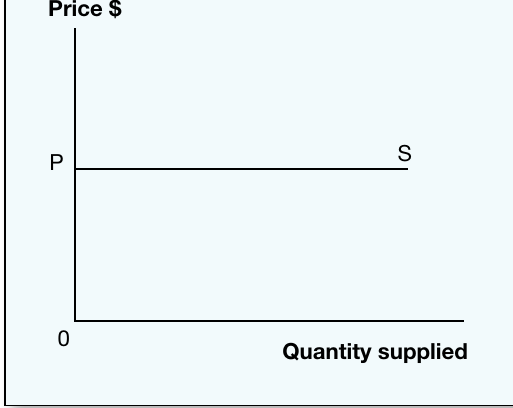
At price P, suppliers would theoretically supply an unlimited quantity. Below that price, quantity supplied falls to zero. In reality, this situation is highly unlikely to occur, as no firm can produce infinite output. However, it represents the theoretical extreme of maximum responsiveness.

Perfectly inelastic supply

Perfectly inelastic supply occurs when producers supply a fixed quantity regardless of the price level. This is represented by a vertical supply curve.

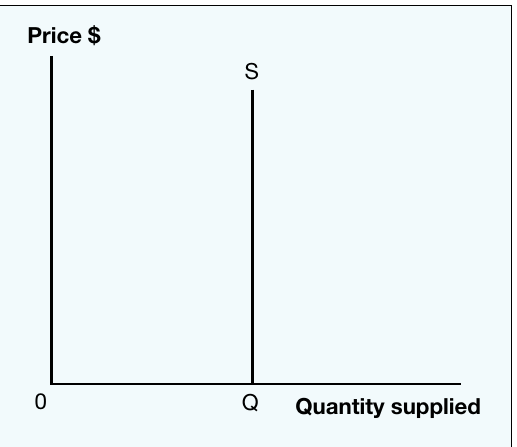
The quantity supplied remains fixed at Q, no matter how much price changes. A real-world example might be a unique piece of art. If only one original painting exists, the supply is fixed at one unit regardless of how high the price rises. Similarly, land in a specific location has perfectly inelastic supply in the short run.

Between the extremes

Most real-world supply curves fall somewhere between these two theoretical extremes. The actual elasticity depends on several factors, which we explore in the next section.

Factors affecting elasticity of supply

Several key factors determine how elastic or inelastic supply will be for a particular product.

Time lags after a price change

The amount of time producers have to respond to a price change is perhaps the most important determinant of elasticity. Generally, the longer the time period, the more elastic supply becomes.

Immediate period: In the very short run, immediately after a price change, supply is virtually perfectly inelastic. Producers cannot adjust any inputs quickly. They can only try to work existing staff and equipment harder, which has limited impact on output.

Short run: Over several weeks or months, producers can vary some inputs to the production process. They can hire additional workers, order more raw materials, or increase overtime. Supply becomes somewhat more responsive, though it remains relatively inelastic because major constraints (like factory size) remain fixed.

Long run: Given sufficient time (months or years), producers can adjust all inputs. They can build new factories, install additional machinery, and fully expand their productive capacity. This makes supply relatively elastic, as firms can substantially increase output in response to higher prices.

The ability to hold and store stock

The ease with which producers can hold inventory affects how readily they can respond to price changes.

Inventory refers to the total stock of finished goods and services held by a firm, which is intended for sale to consumers.

Products that are easy to store can be withheld from the market when prices fall and released when prices rise. This makes supply more elastic. For example:

• Durable goods like furniture, appliances, or tinned food can be stored easily, making their supply relatively elastic
• Non-perishable manufactured goods can be warehoused for extended periods

Conversely, goods that are difficult or impossible to store have more inelastic supply:

• Fresh fruit, vegetables, and dairy products perish quickly
• Services like haircuts or restaurant meals cannot be stored at all
• Live entertainment cannot be inventoried

Excess capacity

Excess capacity exists when a firm is not using its existing resources to full capacity. This concept directly impacts supply elasticity.

When firms have excess capacity (spare resources), supply tends to be elastic. They can quickly increase output by utilizing unused machinery, hiring idle workers, or increasing shifts. For example, a factory running at 50% capacity could potentially double output rapidly in response to a price increase.

When firms are operating at or near full capacity, supply becomes inelastic. There is no spare productive capacity to tap into, so output cannot increase substantially even if prices rise. The firm would need to invest in new capacity (which takes time) to increase production further.

Exam guidance

Summary