Exponential Functions and Models Revision Notes for HSC SSCE Mathematics Standard

Exponential Functions and Models

Understanding exponential functions

An exponential function is a mathematical relationship where the variable appears as the power (or exponent) of a constant number. Unlike other functions you may have studied, exponential functions have the independent variable $x$ in the exponent position.

The general forms of exponential functions are:

$y = a^x$
$y = a^{-x}$

where the constant $a$ must be greater than zero ( $a > 0$ ).

For example, $y = 3^x$ and $y = 2^{-x}$ are both exponential functions.

infoNote

The key distinguishing feature of exponential functions is that the variable appears in the exponent, not as the base. This is what creates their characteristic curved shape and rapid growth or decay behavior.

Graphs of exponential functions

Exponential graphs have distinctive shapes depending on whether the base is in the form $a^x$ or $a^{-x}$ , and whether the base value is greater than 1 or between 0 and 1.

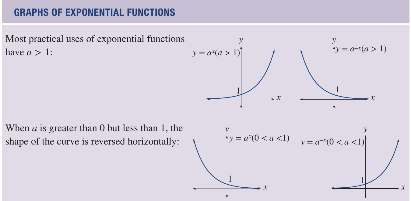
When $a > 1$ :

The function $y = a^x$ creates a growth curve that rises steeply as $x$ increases
The function $y = a^{-x}$ creates a decay curve that falls as $x$ increases

When $0 \< a \< 1$ :

The shapes reverse horizontally compared to when $a > 1$

Special case: When $a = 1$ , the graph becomes a horizontal line at $y = 1$ .

Key features of exponential graphs

Understanding these essential characteristics will help you sketch and interpret exponential graphs:

chatImportant

Critical Characteristics of Exponential Graphs:

These seven features are fundamental to identifying and working with exponential functions. Master these properties to confidently analyze any exponential graph.

1. Always positive outputs

Exponential graphs sit completely above the x-axis. The output value $a^x$ is always positive, regardless of what value $x$ takes. This means y-values can never be zero or negative.

2. Y-intercept at (0, 1)

Every exponential graph passes through the point (0, 1). This is because when $x = 0$ , we have $y = a^0 = 1$ , which is true regardless of the base value $a$ .

3. Asymptotic behaviour

The x-axis acts as an asymptote for exponential graphs. This means the curve gets closer and closer to the x-axis but never actually touches or crosses it.

4. Reflection symmetry

The graph of $y = a^{-x}$ is the reflection of $y = a^x$ in the y-axis. If you folded the page along the y-axis, these two curves would match up.

5. Effect of changing the base

Increasing the base value (for example, changing from $y = 2^x$ to $y = 3^x$ ) makes the graph steeper. The y-values increase more quickly as x increases.

6. Growth functions

When $a > 1$ , the function $y = a^x$ is called a growth function because as x-values increase, y-values also increase.

7. Decay functions

When $a > 1$ , the function $y = a^{-x}$ is called a decay function because as x-values increase, y-values decrease.

How to graph an exponential function

Follow these four steps to sketch an exponential graph:

Create a table of values: Choose several x-values (typically including negative, zero, and positive values) and calculate the corresponding y-values using the exponential function.
Draw a coordinate plane: Set up axes with appropriate scales to accommodate your calculated values.
Plot the points: Mark each coordinate pair from your table on the graph.
Join the points with a smooth curve: Draw a smooth, continuous curve through the points. Remember that exponential graphs are curved, not straight lines.

infoNote

Graphing Tip: Always include $x = 0$ in your table of values. Since all exponential graphs pass through (0, 1), this point serves as a useful reference when sketching the curve.

Exponential models in real-world situations

We use exponential models when a practical situation can be represented mathematically by an exponential function. These situations typically involve quantities that experience fast growth or decay over time.

Exponential growth models

These describe quantities that increase rapidly. The general form is $y = a^x$ where $a > 1$ . Examples include:

Population growth
Compound interest
Spread of diseases
Technology adoption

Exponential decay models

These describe quantities that decrease rapidly. The general form is $y = a^{-x}$ where $a > 1$ . Examples include:

Radioactive decay
Depreciation of assets
Medication concentration in the bloodstream
Temperature cooling

infoNote

Real-World Connection: Exponential models are powerful because they accurately describe many natural and human-made processes. The key indicator that an exponential model is appropriate is when the rate of change is proportional to the current amount.

Worked example: Fish population model

Let's examine a complete example of exponential growth modelling to see how we apply these concepts in practice.

lightbulbExample

Worked Example: Modelling Fish Population Growth

The fish population in a lake is predicted using the formula $N = 500 \times 1.5^t$ , where $N$ is the number of fish and $t$ is the time in years.

Part a: Construct a table of values for $t$ and $N$ using values for $t$ from 0 to 4. Round the number of fish to the nearest whole number.

Solution:

To create the table, substitute each value of $t$ into the formula:

When $t = 0$ : $N = 500 \times 1.5^0 = 500 \times 1 = 500$
When $t = 1$ : $N = 500 \times 1.5^1 = 500 \times 1.5 = 750$
When $t = 2$ : $N = 500 \times 1.5^2 = 500 \times 2.25 = 1125$
When $t = 3$ : $N = 500 \times 1.5^3 = 500 \times 3.375 = 1688$ (rounded)
When $t = 4$ : $N = 500 \times 1.5^4 = 500 \times 5.0625 = 2531$ (rounded)

$t$	0	1	2	3	4
$N$	500	750	1125	1688	2531

Part b: Draw the graph of $N = 500 \times 1.5^t$ .

Solution:

Set up a coordinate plane with $t$ on the horizontal axis (representing time in years) and $N$ on the vertical axis (representing the number of fish).

Plot the five points from the table: $(0, 500)$ , $(1, 750)$ , $(2, 1125)$ , $(3, 1688)$ , and $(4, 2531)$ .

Join these points with a smooth curve to show the exponential growth pattern.

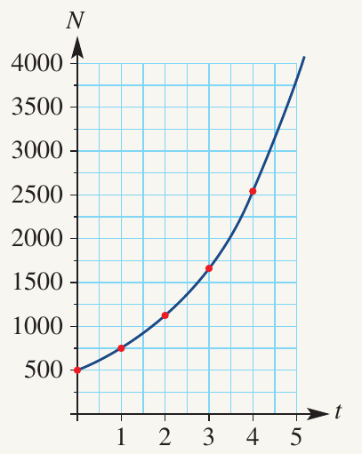
Part c: How many fish were present after 2 years?

Solution:

Look at the table when $t = 2$ and find the corresponding value of $N$ .

Answer: 1125 fish

Part d: How many extra fish will be present after 4 years compared to 2 years?

Solution:

Subtract the population at 2 years from the population at 4 years:

Extra fish $= 2531 - 1125 = 1406$ fish

Answer: 1406 extra fish

Part e: Estimate the number of fish after 18 months.

Solution:

18 months equals 1.5 years, so we need to find $N$ when $t = 1.5$ .

Looking at the graph, when $t = 1.5$ , the curve passes through approximately $N = 900$ .

Answer: Approximately 900 fish

chatImportant

Exam Tip: When reading values from an exponential graph, remember that the curve gets steeper as it rises. Values between plotted points should follow the curve's shape, not a straight line.

bookmarkSummary

Key Points to Remember:

Exponential functions have the form $y = a^x$ or $y = a^{-x}$ where $a > 0$ , with the variable appearing in the exponent.
All exponential graphs pass through the point (0, 1) and stay completely above the x-axis (always positive y-values).
Growth functions ( $y = a^x$ when $a > 1$ ) increase as x increases, while decay functions ( $y = a^{-x}$ when $a > 1$ ) decrease as x increases.
The x-axis is an asymptote—the curve approaches it but never touches it.
Exponential models are used for real-world situations involving rapid growth or decay, such as population changes, radioactive decay, or compound interest.

Exponential Functions and Models (HSC SSCE Mathematics Standard): Revision Notes