Equations for Straight-Line Motion with Constant Acceleration Revision Notes for HSC SSCE Physics

Equations for Straight-Line Motion with Constant Acceleration

Introduction to equations of motion

When studying motion with constant acceleration, we can represent the same physical situation in two equivalent ways: using graphs or using algebraic equations. Neither representation is more important than the other—they are simply different models of the same motion.

infoNote

Graphs and algebraic equations are equally valid ways to describe motion. Understanding both methods gives you flexibility in problem-solving and helps build a deeper understanding of the underlying physics.

For motion at constant acceleration, the velocity versus time graph is a straight line. From this graph, we can extract two key pieces of information:

The gradient (slope) represents the acceleration
The area under the graph represents the distance travelled

From these graphical relationships, we can derive simple algebraic equations that represent exactly the same motion as the graphs show.

The three equations of motion

There are three main equations used to describe motion with constant acceleration. Each equation involves four of the five key variables: $u$ , $v$ , $a$ , $t$ , and $s$ .

Understanding the variables

Before we look at the equations, let's define what each symbol represents:

$u$ = initial velocity (the velocity at the start of the time interval)
$v$ = final velocity (the velocity at the end of the time interval)
$a$ = acceleration (the rate of change of velocity)
$t$ = time (the time interval during which the motion occurs)
$s$ = displacement (the distance travelled in a particular direction)

chatImportant

These five variables (often remembered as SUVAT) are the foundation of all kinematics problems. You'll need to know three of them to find the fourth using the appropriate equation.

Equation 1: Relating velocity, acceleration and time

Starting with the basic definition of acceleration for uniformly accelerated motion:

$a = \frac{v}{t}$

This can be rearranged to give:

$v = at$

However, this assumes there is no initial velocity. To account for an initial velocity (which could still be zero), we add the term $u$ to represent the starting velocity. The final velocity will be the sum of the initial velocity plus the change in velocity due to acceleration:

Equation 1: $v = u + at$

infoNote

This equation is useful when you know the initial velocity, acceleration, and time, and need to find the final velocity. It's the most straightforward of the three equations and is often your first choice when time is known.

Equation 2: Relating displacement, velocity, acceleration and time

To find the displacement (distance travelled), we need to calculate the area under the velocity-time graph.

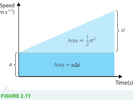
On a velocity-time graph:

The height of the graph represents velocity ( $v$ )
The base represents time ( $t$ )
The area represents displacement ( $s$ )

For constant velocity, displacement would simply be $s = vt$ (the area of a rectangle). However, for uniformly accelerated motion starting with initial velocity $u$ , the graph shows two distinct regions:

A rectangle with area = $u \times t$ (representing the displacement due to the initial velocity)
A triangle on top with area = $\frac{1}{2} \times at \times t$ (representing the additional displacement due to acceleration)

Since $a = \frac{v}{t}$ , which means $v = at$ , the area of the triangle becomes:

$\text{Area of triangle} = \frac{1}{2} \times at \times t = \frac{1}{2}at^2$

The total displacement is the sum of both areas:

Equation 2: $s = ut + \frac{1}{2}at^2$

infoNote

This equation allows you to calculate displacement when you know the initial velocity, acceleration, and time. It's particularly powerful because it gives you position directly, without needing to calculate final velocity first.

Equation 3: Relating velocity, acceleration and displacement

Sometimes you need to relate velocities, acceleration, and displacement without knowing the time interval. By making $t$ the subject of Equation 1 and substituting this into Equation 2, we can derive a third equation that is independent of time:

Equation 3: $v^2 = u^2 + 2as$

chatImportant

Choose this equation when time is unknown and not required! This is the only equation that doesn't involve time, making it perfect for problems where you know velocities, acceleration, and displacement.

Using the equations to solve problems

Each of the three equations involves four of the five kinematic variables. When solving problems:

Identify the known variables from the information given
Identify which variable you need to find
Choose the equation that contains the three known variables and the one unknown variable
Substitute the values carefully, including units
Calculate the answer and express it with appropriate significant figures and units

Once you have found the fourth variable, you can use another equation to find the fifth variable if needed.

lightbulbExample

Worked Example: Car Acceleration (Part 1)

Problem: A car is travelling along a straight road at $20 \text{ m s}^{-1}$ . It accelerates at a uniform $2 \text{ m s}^{-2}$ for $10$ seconds. What is the car's final velocity?

Solution:

Given data:

$u = 20 \text{ m s}^{-1}$ (initial velocity)
$a = 2 \text{ m s}^{-2}$ (acceleration)
$t = 10 \text{ s}$ (time)

We need to find: $v$ (final velocity)

Since we know $u$ , $a$ , and $t$ , we use Equation 1:

$v = u + at$

Substituting values:

$v = 20 \text{ m s}^{-1} + 2 \text{ m s}^{-2} \times 10 \text{ s}$

$v = 20 \text{ m s}^{-1} + 20 \text{ m s}^{-1}$

$v = 40 \text{ m s}^{-1}$

The car's final velocity is 40 m s⁻¹

lightbulbExample

Worked Example: Car Acceleration (Part 2)

Problem: Using the same scenario, what is the total distance travelled by the car during its acceleration phase?

Solution:

Given data:

$u = 20 \text{ m s}^{-1}$
$a = 2 \text{ m s}^{-2}$
$t = 10 \text{ s}$

We need to find: $s$ (displacement)

Since we know $u$ , $a$ , and $t$ , we use Equation 2:

$s = ut + \frac{1}{2}at^2$

Substituting values:

$s = 20 \text{ m s}^{-1} \times 10 \text{ s} + \frac{1}{2} \times 2 \text{ m s}^{-2} \times (10 \text{ s})^2$

$s = 200 \text{ m} + \frac{1}{2} \times 2 \text{ m s}^{-2} \times 100 \text{ s}^2$

$s = 200 \text{ m} + 100 \text{ m}$

$s = 300 \text{ m}$

The car travels a total distance of 300 m during acceleration

lightbulbExample

Worked Example: Using Graphs and Multiple Calculations

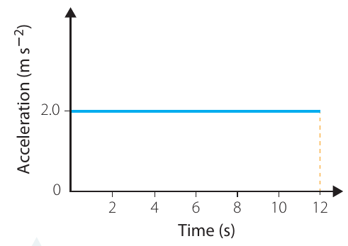
Problem: A car initially travelling at a speed of $4.0 \text{ m s}^{-1}$ accelerates at $2.0 \text{ m s}^{-2}$ for $12$ seconds.

Sketch the acceleration versus time graph
Find the velocity of the car after $8.0$ seconds
Sketch the velocity versus time graph
Find the distance moved by the car in the $8.0$ seconds

Solution:

Part 1: The acceleration is constant at 2.0 m s⁻², so the graph is a horizontal line.

Part 2: The change in velocity equals the area under the acceleration-time graph:

$\Delta v = 2.0 \text{ m s}^{-2} \times 8.0 \text{ s} = 16 \text{ m s}^{-1}$

The final velocity is:

$v = u + \Delta v = 4.0 \text{ m s}^{-1} + 16 \text{ m s}^{-1} = 20 \text{ m s}^{-1}$

Part 3: The velocity increases linearly from $4.0 \text{ m s}^{-1}$ to $20 \text{ m s}^{-1}$ over $8.0$ seconds.

Part 4: The distance equals the area under the velocity-time graph. Using the trapezium formula:

$s = \frac{1}{2}(u + v) \times t = \frac{1}{2}(4.0 \text{ m s}^{-1} + 20 \text{ m s}^{-1}) \times 8.0 \text{ s}$

$s = \frac{1}{2} \times 24 \text{ m s}^{-1} \times 8.0 \text{ s} = 96 \text{ m}$

The car moves 96 m in the 8.0 seconds

Graphical versus algebraic analysis

Both graphical and algebraic methods yield the same answers because they are both models of the same physical motion.

Graphical analysis is often simpler and more intuitive. Once you sketch a velocity versus time graph with the relevant data points:

Acceleration can be found from the gradient (slope)
Distance can be calculated from the area under the curve

Algebraic analysis using the equations is systematic and precise, particularly useful for complex calculations where graphical methods might be less accurate.

infoNote

Choose the method that best suits the problem and the information given. In exams, you may be required to demonstrate both methods, so practice with each approach.

Linear acceleration under gravity

What is gravitational acceleration?

Once an object is released or thrown, the only significant force acting on it (ignoring air resistance) is the gravitational force. Near Earth's surface, gravity causes all objects to accelerate vertically downwards with an acceleration of approximately:

$g = 9.8 \text{ m s}^{-2}$

This value is called gravitational acceleration and is given the symbol $g$ . Although $g$ varies slightly around the world, using $9.8 \text{ m s}^{-2}$ gives sufficiently accurate answers for most purposes.

chatImportant

All objects fall at the same rate in the absence of air resistance, regardless of their mass. This was famously demonstrated by Apollo 15 astronaut Commander David Scott, who dropped a hammer and a feather on the Moon. With no atmosphere to provide air resistance, both objects hit the ground simultaneously.

Understanding "metres per second per second"

The value $9.8 \text{ m s}^{-2}$ is read as "9.8 metres per second per second." This means that for every second an object falls, its speed increases by 9.8 m s⁻¹.

For example:

After $1$ second: velocity = $9.8 \text{ m s}^{-1}$ (about $35 \text{ km h}^{-1}$ )
After $2$ seconds: velocity = $19.6 \text{ m s}^{-1}$ (about $70 \text{ km h}^{-1}$ )
After $10$ seconds: velocity = $98 \text{ m s}^{-1}$ (about $350 \text{ km h}^{-1}$ )

infoNote

This rapid increase in speed explains why falling from even moderate heights can be dangerous. After just 3 seconds of free fall, an object is already moving at nearly 30 m s⁻¹ (about 108 km h⁻¹)!

Graphs for falling objects

When an object is dropped from rest, its motion can be represented by three graphs:

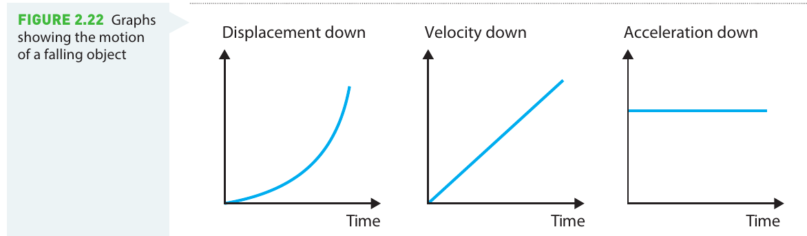
Displacement-time graph: Shows a parabolic curve (displacement increases at an increasing rate)
Velocity-time graph: Shows a straight line through the origin (velocity increases uniformly)
Acceleration-time graph: Shows a horizontal line (acceleration is constant at $g$ )

Objects falling directly downwards

When analysing falling objects, we typically set the origin at the point where the object starts to move. If we define the downward direction as positive, then all variables ( $s$ , $u$ , $v$ , $a$ , and $t$ ) will be positive, with:

$a = g = +9.8 \text{ m s}^{-2}$

The same three equations of motion apply, simply replacing $a$ with $g$ .

chatImportant

Sign convention matters! Be consistent with your choice of positive direction. If you take downward as positive, then $g = +9.8 \text{ m s}^{-2}$ . If you take upward as positive, then $g = -9.8 \text{ m s}^{-2}$ .

lightbulbExample

Worked Example: Watch Falling from a Bridge

Problem: A watch falls from a Sydney Harbour Bridge climber's wrist. The watch falls for $2.5$ seconds before hitting a car below.

Sketch a velocity versus time graph of this motion
With what velocity does the watch hit the car?
How far did the watch fall?

Solution:

Part 1: The velocity-time graph starts at the origin (initial velocity = 0) and increases linearly with a positive gradient.

Part 2:

Given data:

$u = 0$ (starts from rest)
$a = -9.8 \text{ m s}^{-2}$ (if taking downward as negative)
$t = 2.5 \text{ s}$

Using Equation 1:

$v = u + at = 0 + (-9.8 \text{ m s}^{-2}) \times 2.5 \text{ s}$

$v = -24.5 \text{ m s}^{-1}$

The watch hits the car with a velocity of 24.5 m s⁻¹ vertically down.

Part 3:

Using Equation 2:

$s = ut + \frac{1}{2}at^2 = 0 + \frac{1}{2} \times 9.8 \text{ m s}^{-2} \times (2.5 \text{ s})^2$

$s = \frac{1}{2} \times 9.8 \text{ m s}^{-2} \times 6.25 \text{ s}^2$

$s = 31 \text{ m}$

The watch fell a distance of 31 metres (to two significant figures).

Investigation 2.2: Measuring gravitational acceleration

This investigation allows you to experimentally determine the value of $g$ by collecting first-hand data.

Aim

To find the value of gravitational acceleration, g
To investigate average and instantaneous velocities

Materials

Ruler
Ball bearing
Electronic timer or timing photogate

Risk assessment

What are the risks?	How can you safely manage these risks?
The ball bearing may cause injury if thrown, dropped, or stepped on	- Never throw ball bearings - Manage the use of the ball bearing carefully - Never leave the ball bearing on the ground

Method

Set up the electronic timing apparatus
Carefully measure the vertical distance, $s$ , that the ball bearing will fall
Release the ball bearing from rest and measure the time, $t$ , taken to fall through the known height
Repeat this measurement several times to get an average
Change the height and repeat the procedure
Record sufficient data to plot a graph

infoNote

Taking multiple measurements at each height and calculating an average helps reduce the effect of random errors. Aim for at least three measurements at each height.

Results

Record all raw and derived data in a correctly constructed data table
Plot the data as it is collected
Estimate and record uncertainties in the data

Analysis of results

Plot $s$ versus $t_{\text{avg}}$ with uncertainty bars and draw a line of best fit
Create a data table with columns for $t_{\text{avg}}$ , $s$ , $(t_{\text{avg}})^2$ , and $v_{\text{avg}}$
Plot $s$ versus $(t_{\text{avg}})^2$
Draw a straight line of best fit and calculate the gradient
Use the equation $s = ut + \frac{1}{2}at^2$ $s = u t + \frac{1}{2} a t^{2}$ to relate the gradient to $g$ $g$
- Since $u = 0$ for a dropped object: $s = \frac{1}{2}gt^2$
- Therefore, gradient of s vs t² graph = ½g
- So: $g = 2 \times \text{gradient}$
Calculate the best estimate of $g$ from your gradient
Use the maximum and minimum possible gradients to estimate the uncertainty in $g$
Calculate average speed for each $(s, t_{\text{avg}})$ pair: $v_{\text{avg}} = \frac{s}{t}$
Plot $v_{\text{avg}}$ versus $s$ and describe the trend

chatImportant

Exam tip: When calculating gradients for experimental data, always draw a line of best fit and use two points on that line—do not simply use two data points. This reduces the effect of random errors.

bookmarkSummary

Key Points to Remember:

There are three main equations for constant acceleration: $v = u + at$ , $s = ut + \frac{1}{2}at^2$ , and $v^2 = u^2 + 2as$
Choose the equation that contains the three known variables and the one unknown you need to find
Graphical and algebraic methods are equivalent—both give the same answer for the same motion
On a velocity-time graph: gradient = acceleration and area = displacement
Gravitational acceleration $g = 9.8 \text{ m s}^{-2}$ causes all objects to fall at the same rate (in the absence of air resistance)
Always include units in your calculations and express answers with appropriate significant figures

Equations for Straight-Line Motion with Constant Acceleration (HSC SSCE Physics): Revision Notes