Transition Matrices – Using Recursion (VCE SSCE General Mathematics): Revision Notes
Transition Matrices – Using Recursion
Introduction to matrix recurrence relations
A recurrence relation is a mathematical method for modelling systems that change over time. You may have encountered recurrence relations when studying financial modelling, such as calculating compound interest year by year. The same principle applies to transition matrices, but now we work with matrices instead of single values.
The concept of recurrence relations extends beyond financial modelling. Whenever a system evolves step-by-step based on its previous state, we can use recurrence relations to model and predict its behavior.
When using transition matrices with recursion, we track how a system evolves through successive states. Each state is represented by a state matrix, and we use a transition matrix to move from one state to the next.
Key components
Every matrix recurrence relation requires:
- An initial state matrix () representing the starting conditions
- A transition matrix () showing how the system changes
- A recurrence rule that generates each successive state
The beauty of this method is that it allows us to predict future states of complex systems through straightforward matrix multiplication.
The matrix recurrence relation formula
The fundamental formula for matrix recurrence relations is:
This formula tells us that to find the state at step , we multiply the transition matrix by the current state matrix .
Understanding the notation
- represents the initial state (at time 0)
- represents the state after one transition
- represents the state after two transitions
- represents the state after transitions
- is the transition matrix that remains constant
Generating state matrices step-by-step
Let's examine how to generate successive state matrices using the car rental example. A rental company has cars distributed between two locations: Bendigo and Colac. Initially, there are 50 cars in Bendigo and 40 in Colac.
The transition matrix is:
The initial state matrix is:
Calculating (state after 1 week)
To find the distribution after one week, we calculate:
After 1 week, there will be 44 cars in Bendigo and 46 in Colac.
Calculating (state after 2 weeks)
Using the same approach:
After 2 weeks, there will be 39.8 cars in Bendigo and 50.2 in Colac.
Calculating (state after 3 weeks)
Continuing the pattern:
After 3 weeks, there will be 36.9 cars in Bendigo and 53.1 in Colac.
Recognising the pattern
From these calculations, we can see the pattern emerging:
Pattern Recognition
More generally:
This recurrence relation enables us to model the system step-by-step. Each state depends only on the previous state and the transition matrix.
Worked example: Factory machines using recursion
Worked Example: Factory Machine States
A factory has 100 machines that can be in one of two states: operating () or broken (). Initially, 80 machines are operating and 20 are broken.
Given:
We need to find the state after 1 day and after 3 days.
Finding the state after 1 day
Using :
After 1 day, 69 machines are operational and 31 are broken.
Finding the state after 3 days
First, we need :
Then we can find :
After 3 days, approximately 53 machines are operating and 47 are broken.
Direct calculation method: Finding efficiently
While the step-by-step method works well for small values of , it becomes tedious for large values. There is a more efficient method for finding the state after steps without calculating all intermediate states.
Deriving the direct formula
Let's follow the pattern algebraically:
Continuing this pattern:
This gives us the general formula:
This formula allows us to jump directly to any future state without calculating intermediate steps.
When to Use Each Method
- Use when you need to see the progression step-by-step or when working with small values of
- Use when you need to find a specific future state quickly
- The direct method is especially useful for large values of (e.g., )
Worked example: Using the direct formula
Worked Example: Factory State After 10 Days
Using the same factory problem, let's find the state after 10 days directly.
Given:
Solution
Using the formula with :
Using a calculator to compute :
After 10 days, approximately 31 machines will be operational and 69 will be broken.
This calculation, which would have required 10 separate matrix multiplications using the step-by-step method, can be done in one operation using the direct formula.
Using inverse matrices to find previous states
Sometimes we need to work backwards through the sequence of states. For example, if we know the state at step but need to find the state at step , we can use the inverse of the transition matrix.
The inverse relationship
We know that:
By multiplying both sides by :
Therefore:
This allows us to move backwards through the state sequence.
Important Note About Inverse Matrices
The inverse matrix is generally not itself a transition matrix. It's simply a mathematical tool for reversing the process. The elements of may not represent probabilities and may even be negative or greater than 1.
Worked example: Finding previous states
Worked Example: Working Backwards Through States
Given a transition matrix:
And we know that:
We need to find and .
Solution
First, calculate the inverse matrix:
Finding :
Finding :
Alternatively, we could have calculated directly using:
The steady-state solution
One of the most important questions when analysing transition matrices is: "What happens in the long term?" Often, systems don't continue changing indefinitely. Instead, they settle down to a steady state or equilibrium state where the values remain constant.
What is a steady state?
A steady state occurs when the state matrix stops changing, even though transitions continue to happen. The values stabilize at fixed amounts.
For the car rental problem, let's examine what happens over 15 weeks:
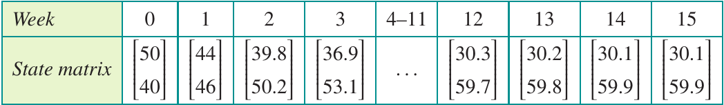
Notice that:
- Initially, the values change significantly each week
- After several weeks, the changes become smaller
- Eventually, the values stabilize at approximately 30 cars in Bendigo and 60 in Colac
- Once reached, these values don't change
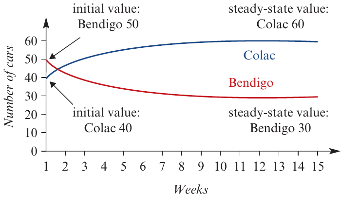
The graph shows this convergence visually. Both locations' car numbers approach fixed values and remain there.
Understanding equilibrium
The term "equilibrium" is particularly apt because, even though cars are still moving between locations in the steady state, the flows are balanced. The number of cars leaving Bendigo for Colac equals the number leaving Colac for Bendigo. This balance maintains the steady-state values.
What Equilibrium Really Means
At equilibrium, the system isn't static—transitions are still occurring. However, the inflows and outflows for each state are perfectly balanced, so the overall distribution remains constant. Think of it like a bathtub with water flowing in and out at the same rate—the water level stays constant.
Conditions for a steady state
Two Essential Conditions for Steady State
For a system to have a steady-state solution, two conditions must be met:
-
The transition matrix must be regular: A regular matrix is one whose powers never contain any zero elements. In practical terms, this means every state must be accessible (either directly or indirectly) from every other state.
-
The columns must sum to 1: This ensures that probabilities are properly normalized and the total of all quantities is conserved.
When these conditions are met, the system will converge to a steady state regardless of the initial state matrix.
Estimating the steady-state solution
While we can observe steady-state values by calculating many successive state matrices, there's a more efficient approach using the direct formula.
The steady-state formula
If is the initial state matrix, the steady-state matrix is given by:
as tends to infinity ().
In practice, we cannot calculate , but we can approximate the steady state by using large values of . Depending on the system, values like often give excellent approximations.
How to verify convergence
To confirm that a steady state has been reached to a given degree of accuracy, check that at least two successive state matrices agree to that accuracy. For example, if and both round to the same values, the steady state has been reached.
Choosing the Right Value of n
Different systems converge at different rates. If the values are still changing noticeably, try larger values of . Always compare successive states (like and ) to verify convergence rather than assuming a particular is sufficient.
Worked example: Estimating steady state
Worked Example: Finding the Steady-State Distribution
For the car rental problem with:
Let's estimate the steady-state solution by calculating for .
Solution
Using :
For :
For :
For :
For :
Conclusion
Since and agree to one decimal place, the steady-state solution has been reached. The steady-state distribution is approximately 30 cars in Bendigo and 60 cars in Colac.
This confirms the result we observed earlier through step-by-step calculation, but achieves it much more efficiently.
Using technology: Calculator methods
Modern calculators can greatly simplify recurrence relation calculations. Here's how to use a CAS calculator effectively:
Calculator Setup and Tips
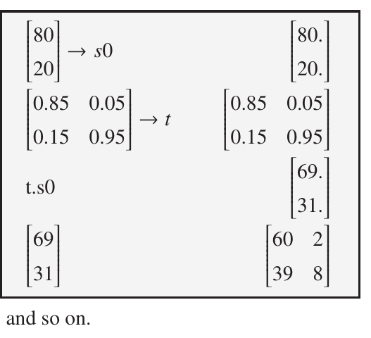
Setting up matrices
Store your initial state matrix as a variable (e.g., s0 or S) and your transition matrix as another variable (e.g., t or T).
For example:
Calculating successive states
To find , simply enter: t · s0
To find , enter: t^10 · s0
The calculator handles all matrix multiplication automatically.
Benefits of using technology
- Eliminates arithmetic errors
- Speeds up calculations significantly
- Allows easy experimentation with different values of
- Makes it practical to find steady states quickly
Summary
Key Points to Remember:
-
Matrix recurrence relations follow the pattern: ,
-
Direct calculation using is more efficient for finding specific future states
-
Inverse matrices allow backward calculation:
-
Steady states occur when the system stabilizes at fixed values that no longer change
-
Regular matrices with columns summing to 1 will converge to a steady state
-
Estimate steady states by calculating for large values of
-
At equilibrium, flows are balanced even though transitions continue
-
Verify convergence by checking that successive state matrices agree to the required accuracy